Unhide Columns in Excel: Easy Methods and Pro Tips

Hiding columns is a very common technique when working with Excel spreadsheets. This makes sense for readability purposes: You may want to focus on certain metrics, or you may want to remove unnecessary information in your data views.

Whatever the reason, while hiding columns is fairly easy, unhiding them can be, surprisingly, a bit more complicated. Don't worry - in this article, we will have a look at the available methods to unhide columns, including shortcuts and some good tips to make unhiding columns and managing grouped columns extremely easy.

How to Unhide Columns in Excel: Basic Methods

Let’s start with the most basic methods to unhide columns in Excel. 

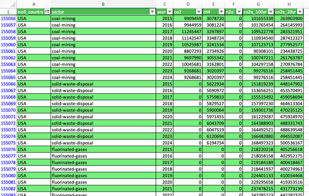
We will use a database with greenhouse gas emissions by country, sector, and year, prepared by Climate Trace. The data looks like this:

Using the right-click menu

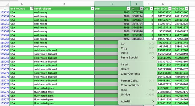
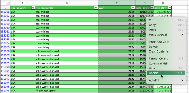
The simplest way to unhide columns is by selecting the columns located next to the hidden columns and then clicking on the Unhide button in the right-click menu. 

In the following image, we unhide the column “co2”.

Using the Format menu

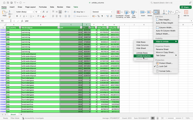
Alternatively, you can unhide columns from the Home menu. Just select the adjacent columns first and then go to Home > Format > Hide & Unhide > Unhide Columns, as shown below:

Using the drag method

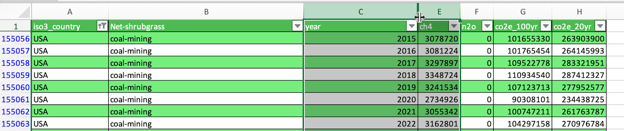
It’s also possible to do the trick by hovering between the adjacent column letters and then double-clicking or dragging to reveal hidden columns.

Using keyboard shortcuts

Finally, we unhide columns using keyboard shortcuts. In the case of Windows, you can do this in two ways:

• Alt + H + O + U + L: This sequence opens the Excel ribbon to Unhide Columns.
• Ctrl + Shift + 0: This is the primary shortcut for unhiding columns in Excel. 

Special Case: Unhiding the First Column (Column A)

If the first column (column A) is hidden, it can be a bit tricky because there’s no straightforward way to select the column in the spreadsheet. Let’s see several ways to address this situation.

Using the Name Box

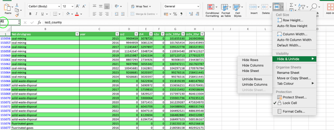
An easy way to point to the hidden column A is by using the Name Box in the upper left corner. Just type A1 and then go to Home > Format > Hide & Unhide > Unhide Columns.

Using the Go To command

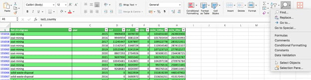
Similarly, you can go A1 through the Go To command. Just follow Home > Find & Select > Go To, enter A1, and proceed as in the last section.

Dragging from column B

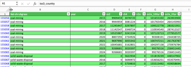
Finally, you can also unhide column A by carefully dragging to the left from column B, as shown below.

How to Unhide All Columns at Once

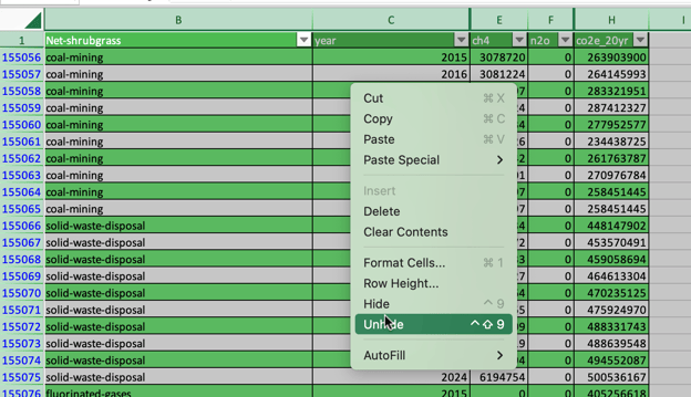
It may happen that you have multiple, non-consecutive hidden columns in your worksheet. If you want to unhide all of them at once, first, select the entire sheet (either by using Ctrl + A twice or clicking the triangle at the top-left, and then follow the usual right-click > Unhide or Format > Hide & Unhide > Unhide Columns.

How to Unhide Specific Multiple Columns

Unhiding specific multiple columns follows the same logic. Just select the range that spans the hidden columns and then proceed with the standard unhide steps. 

How to Find Hidden Columns in Excel

Sometimes, hidden columns are hard to locate. Here are two methods to help:

Using Go To Special to find hidden columns

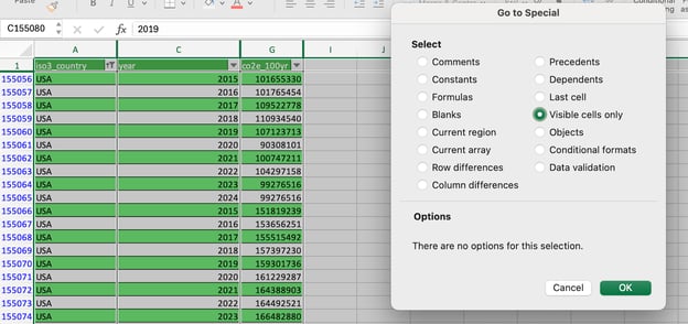
When working in spreadsheets with many columns, it may be difficult to identify at first sight all the hidden columns. A great method to do this is by following Home > Find & Select > Go To Special > Visible cells only. As a result, Excel will highlight with a thicker line the borders between column and column names where there are hidden columns.

Using Document Inspector to check for hidden columns

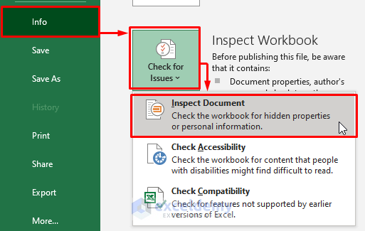
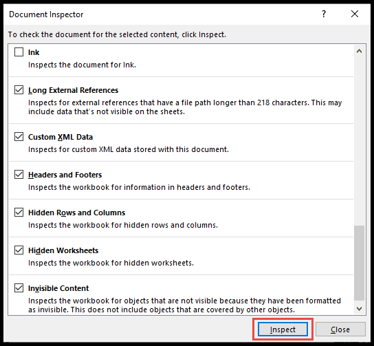
If you’re using Excel in Windows, you can also check the hidden columns in your worksheet through the Document Inspector. Just go to File > Info > Check for Issues > Inspect Document and click on Hidden Rows and Columns to get a view of the total hidden rows and columns.

How to Prevent Others from Unhiding Columns

Finally, you may want to protect your worksheet by limiting the possibility of other users unhiding columns. This may be necessary if the documents contain information that not everyone in the company is allowed to see. 

This process takes several steps. First, select all cells with Ctrl + A twice or click on the triangle at the top-left. Then, press Ctrl + 1 to display the Format Cell box. Go to Protection, and you will see that cells are locked by default. This constraint only applies when you protect your worksheet (see below). Uncheck the Locked status for now.

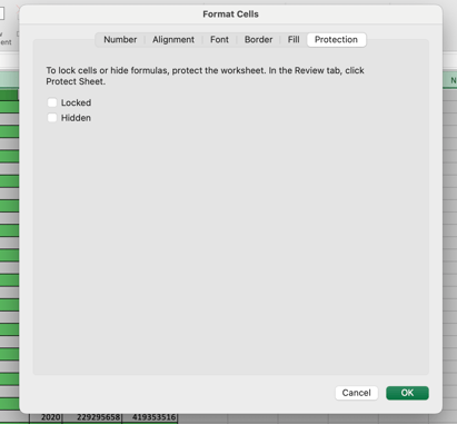
Now, select the columns you want to hide and press Ctrl + 1 again. Go to the Protection tab and enable the Locked option.

Finally, go to Review > Protect your Sheet and allow users only to select unlocked cells. Make sure the Select locked cells is disabled.

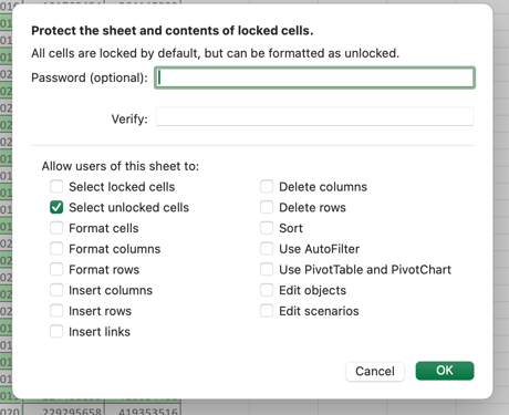
Now, your users cannot manipulate or unhide the hidden columns. However, this formula is not bulletproof, as users could still access information on the hidden columns through a formula.

Conclusion

Unhiding columns in Excel may seem a trivial task, but it’s important to know how to do it to prevent confusion and ensure high readability. We have covered all the available options for different use cases, including pro tips for more complex scenarios, such as collaborative worksheets.

We hope you enjoyed this tutorial and look forward to seeing you again. In the meantime, we are here to help you become an Excel master. Check out other compelling Excel materials we have for you:

• Introduction to Excel course
• Data Analysis in Excel course
• Excel Fundamentals skill track