Hồi quy đa thức: Từ đường thẳng đến đường cong

Khi dữ liệu của bạn uốn cong, việc dùng một đường thẳng để ước lượng các điểm dữ liệu mới là không hợp lý. Làm vậy, bạn sẽ có một mô hình bỏ lỡ quy luật, có sai số dư cao và dự đoán kém. Dữ liệu thế giới thực hiếm khi tuyến tính, dù bạn đang mô hình hóa cách liều lượng thuốc ảnh hưởng đến đáp ứng, cách nhiệt độ tác động lên ứng suất vật liệu, hay cách giá tài sản biến động theo thời gian.

Hồi quy đa thức khắc phục điều này bằng cách mở rộng hồi quy tuyến tính để khớp các đường cong thay vì đường thẳng. Chỉ cần thêm vài hạng bậc cao hơn - x², x³ - và mô hình của bạn có thể theo sát hình dạng thực sự của dữ liệu.

Trong bài viết này, tôi sẽ trình bày hồi quy đa thức là gì, toán học đằng sau nó, cách triển khai bằng Python, và cách tránh chiếc bẫy mà nhiều người mắc phải: quá khớp.

Nếu bạn còn mới với khái niệm học máy, hãy đọc trước hướng dẫn Những điều cốt yếu của Hồi quy Tuyến tính trong Python trước.

Hồi quy đa thức là gì?

Hồi quy đa thức là thuật toán bạn nên dùng khi một đường thẳng không thể mô tả dữ liệu của bạn.

Hồi quy tuyến tính mô hình hóa mối quan hệ giữa các biến dưới dạng một đường thẳng. Cách này hiệu quả khi mối quan hệ thực sự là tuyến tính - nhưng phần lớn dữ liệu thực tế thì không. Hãy nghĩ đến cách quãng đường phanh của ô tô thay đổi theo tốc độ, hay tốc độ sinh trưởng của cây phản ứng với phân bón. Những mối quan hệ này uốn cong. Một đường thẳng sẽ không khớp tốt, dù bạn làm gì.

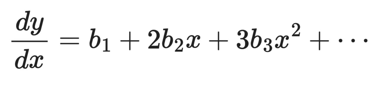
Hồi quy đa thức mở rộng hồi quy tuyến tính bằng cách thêm các hạng bậc cao hơn vào phương trình. Thay vì khớp y = b0 + b1x, bạn sẽ khớp dạng như y = b0 + b1x + b2x² + b3x³. Bậc của đa thức - chữ n trong "đa thức bậc n" - kiểm soát số lần đường cong có thể uốn lượn.

Nói ngắn gọn và dễ hiểu, đây là khác biệt then chốt giữa hai phương pháp:

• Hồi quy tuyến tính: Khớp một đường thẳng. Mỗi đặc trưng một hệ số, một mức độ tự do trong đường cong.

• Hồi quy đa thức: Khớp một đường cong. Mỗi hạng bổ sung (x², x³, ...) cho mô hình thêm linh hoạt để bám theo hình dạng dữ liệu.

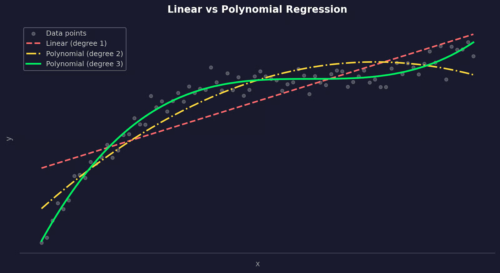
Hồi quy tuyến tính so với hồi quy đa thức

Về bản chất, hồi quy đa thức vẫn là một mô hình tuyến tính. "Tuyến tính" ở đây nói về cách mô hình xử lý các hệ số, không phải hình dạng đường cong tạo ra. Bạn đang thêm các đặc trưng mới (x², x³) và khớp một phương trình tuyến tính trên chúng.

Vậy khi nào thực sự nên dùng?

Hãy chọn hồi quy đa thức khi biểu đồ phần dư từ mô hình tuyến tính cho thấy có quy luật - đó là dấu hiệu mối quan hệ không tuyến tính. Nó cũng phù hợp khi bạn có hiểu biết miền chỉ ra mối quan hệ cong, như trong vật lý, sinh học hoặc kinh tế học.

Đổi lại, các đa thức bậc cao có thể trở nên bất ổn. Đa thức bậc 2 hoặc 3 xử lý được hầu hết các đường cong thực tế, nhưng khi tăng cao hơn, bạn dễ đang khớp nhiễu thay vì tín hiệu.

Vì sao dùng hồi quy đa thức?

Phần lớn các mối quan hệ trong thế giới thực không tuyến tính.

Một đường thẳng có thể tiệm cận, nhưng "tiệm cận" là chưa đủ khi bạn dự đoán những thứ nhạy cảm. Khi mối quan hệ trong dữ liệu uốn cong, mô hình tuyến tính sẽ liên tục bỏ lỡ đoạn uốn đó.

Hồi quy đa thức làm tốt hơn bằng cách cho phép mô hình uốn cong. Thay vì ép một đường thẳng xuyên qua dữ liệu, bạn đang khớp một đường cong có thể bám theo hình dạng của mối quan hệ.

Dưới đây là một số lĩnh vực mà nó tạo ra khác biệt rõ rệt:

• Sinh học và y học: Mối quan hệ liều - đáp ứng hiếm khi tuyến tính. Liều thấp có thể ít tác dụng, liều trung bình hiệu quả, và liều cao gây tác dụng phụ. Đường cong hình chữ S đó cần mô hình đa thức để nắm bắt
• Kỹ thuật: Quan hệ ứng suất - biến dạng của vật liệu, lực cản khí động, và giãn nở nhiệt đều theo các quy luật phi tuyến mà hồi quy đa thức mô hình hóa tốt
• Tài chính: Lợi suất tài sản, định giá quyền chọn, và đường cầu thường thể hiện hiệu ứng giảm dần hoặc tăng dần mà đường thẳng không thể biểu diễn
• Pipeline học máy: Các đặc trưng đa thức là cách nhanh để thêm tính phi tuyến vào mô hình tuyến tính mà không cần chuyển sang thuật toán phức tạp hơn

Điểm chung ở tất cả các trường hợp này là: mối quan hệ giữa đầu vào và đầu ra thay đổi tại các giá trị x khác nhau. Hồi quy tuyến tính giả định sự thay đổi đó là hằng số. Hồi quy đa thức thì không.

Tuy vậy, hồi quy đa thức không phải đũa thần.

Nó hiệu quả nhất khi bạn có hiểu biết miền gợi ý mối quan hệ cong, hoặc khi biểu đồ phần dư rõ ràng cho thấy một quy luật mà đường thẳng không xử lý được. Hãy dùng với một vấn đề cụ thể trong đầu - chứ không chỉ vì R² của mô hình tuyến tính chưa đủ cao.

Hiểu toán học đằng sau hồi quy đa thức

Nắm được toán học cơ bản đằng sau hồi quy đa thức sẽ giúp bạn hiểu nó tốt hơn.

Các hạng đa thức

Trong hồi quy tuyến tính, mô hình của bạn trông như sau:

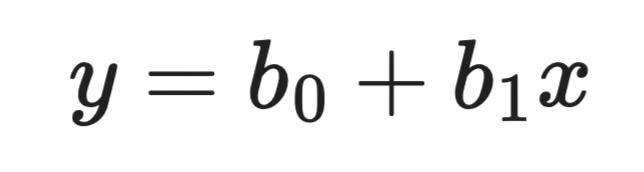
Công thức hồi quy tuyến tính

Đó là một biến đầu vào, một hệ số, một đường thẳng. Hồi quy đa thức mở rộng bằng cách thêm các hạng bậc cao hơn:

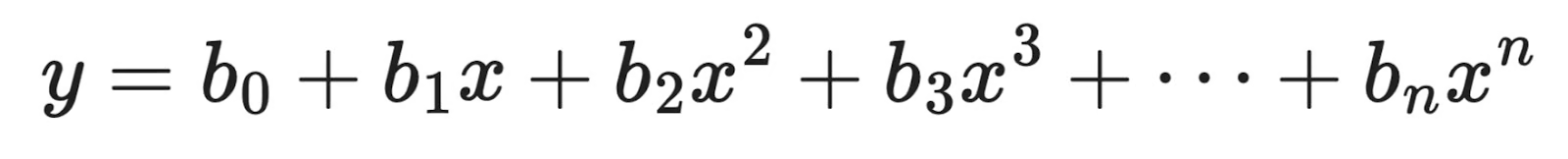
Công thức hồi quy đa thức

Mỗi hạng mới - x², x³, v.v. - cho mô hình thêm một "điểm uốn" để sử dụng. Đa thức bậc 2 có thể khớp một đường cong đơn. Đa thức bậc 3 có thể khớp một đường cong đổi hướng một lần. Bậc n kiểm soát mức độ linh hoạt của mô hình.

Thuật toán nền tảng vẫn giữ nguyên. Bạn chỉ đang thêm các đặc trưng mới. x² được coi như một biến đầu vào riêng, tương tự x. Mô hình vẫn khớp một phương trình tuyến tính - chỉ là trên các đặc trưng đã biến đổi.

Ước lượng bình phương tối thiểu

Việc khớp mô hình hồi quy đa thức hoạt động giống như hồi quy tuyến tính - tức dùng ước lượng bình phương tối thiểu.

Ý tưởng là tìm các hệ số làm tối thiểu tổng bình phương phần dư:

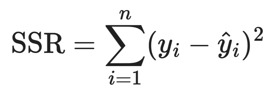
Công thức SSR

Mỗi chênh lệch bình phương là một phần dư - khoảng cách giữa dự đoán của mô hình và quan sát thực tế. Bình phương giúp đảm bảo lỗi âm và dương không triệt tiêu nhau, và phạt lỗi lớn nặng hơn lỗi nhỏ.

Trong thực tế, thư viện sẽ xử lý giúp bạn. Nhưng biết rằng bình phương tối thiểu là mục tiêu sẽ giúp bạn hiểu vì sao điểm ngoại lai gây hại cho mô hình đa thức đến vậy - một phần dư lớn bị bình phương sẽ kéo các hệ số theo hướng của nó.

Diễn giải các hệ số

Trong hồi quy tuyến tính, b1 có cách hiểu đơn giản: mỗi khi x tăng một đơn vị, y thay đổi một lượng b1.

Hồi quy đa thức phức tạp hơn một chút. Khi mô hình của bạn gồm b_1x + b_2x^2, tác động của x lên y phụ thuộc vào giá trị hiện tại của x - bạn không thể đọc b2 một cách tách rời để rút kết luận. Độ dốc của đường cong liên tục thay đổi, điều bạn có thể thấy bằng cách lấy đạo hàm theo x:

Đạo hàm theo x

Bản thân độ dốc là một hàm của x. Điều đó có nghĩa tác động của một thay đổi một đơn vị ở x là khác nhau tại mỗi điểm trên đường cong.

Đây là lý do bạn không nên cố gắng diễn giải từng hệ số riêng lẻ trong mô hình đa thức. Thay vào đó, hãy nhìn toàn bộ đường cong. Vẽ dự đoán của bạn chồng lên dữ liệu.

Ứng dụng của hồi quy đa thức trong khoa học dữ liệu

Hồi quy đa thức xuất hiện ở nhiều lĩnh vực vì các mối quan hệ cong có mặt ở khắp dữ liệu thực tế.

Tài chính

Dữ liệu tài chính hiếm khi di chuyển theo đường thẳng.

Giá tài sản, tăng trưởng doanh thu, và đường cầu đều có xu hướng tăng tốc, giảm tốc, hoặc đảo chiều tùy điều kiện thị trường. Mô hình tuyến tính giả định tốc độ thay đổi là hằng số, điều gần như không bao giờ đúng. Hồi quy đa thức cho phép bạn mô hình hóa các dịch chuyển này - ví dụ, cách nhu cầu người tiêu dùng giảm dần chậm lúc đầu, rồi nhanh chóng khi giá vượt qua một ngưỡng nhất định.

Nó cũng hữu ích cho phân tích xu hướng theo thời gian. Khi bạn khớp một đường cong với dữ liệu giá lịch sử hoặc mô hình hóa cách một chỉ số tăng trưởng qua các giai đoạn chu kỳ kinh doanh, một đa thức bậc 2 hoặc 3 thường ước lượng hình dạng tốt hơn nhiều so với đường thẳng.

Kỹ thuật

Các quá trình vật lý là những ví dụ điển hình về mối quan hệ phi tuyến.

Ứng suất và biến dạng trong vật liệu, động lực học chất lỏng, giãn nở nhiệt, và lực cản khí động đều theo đường cong, không phải đường thẳng. Nhiều phương trình chi phối trong vật lý vốn mang tính đa thức. Hồi quy đa thức cung cấp cách tiếp cận dựa trên dữ liệu để khớp các đường cong đó khi bạn có đo đạc nhưng không có phương trình dạng đóng gọn gàng.

Một ví dụ hay là lực cản, tăng theo bình phương vận tốc. Mô hình tuyến tính sẽ đánh giá thấp lực cản ở tốc độ cao, còn đa thức bậc 2 sẽ khớp đúng mối quan hệ.

Học máy

Trong học máy, hồi quy đa thức thường được dùng như một kỹ thuật kỹ thuật đặc trưng hơn là mô hình độc lập.

Bằng cách thêm các hạng đa thức - x², x³, các hạng tương tác - vào tập đặc trưng, bạn cho mô hình tuyến tính khả năng khớp các quy luật phi tuyến mà không cần chuyển sang thuật toán phức tạp hơn. Đây là bước đầu thường dùng khi mô hình tuyến tính của bạn thiếu khớp và bạn muốn tăng linh hoạt trước khi cân nhắc cây quyết định hay mạng nơ-ron.

Nó cũng hữu ích như một mô hình chuẩn so sánh.

Trước khi huấn luyện mô hình phức tạp hơn, khớp hồi quy đa thức cho bạn biết một đường cong đơn giản có thể giải thích bao nhiêu phương sai. Nếu đa thức bậc 3 đã giải thích được phần lớn, có thể bạn không cần gì phức tạp hơn.

Cách chọn bậc phù hợp cho hồi quy đa thức

Chọn bậc của đa thức là một trong những quyết định quan trọng nhất bạn sẽ đưa ra. Nếu chọn sai theo bất kỳ hướng nào, bạn sẽ có một mô hình kém chính xác.

May mắn thay, chỉ vài dòng Python là đủ để thực hiện.

Quá khớp vs. thiếu khớp

Thiếu khớp xảy ra khi bậc quá thấp. Đa thức bậc 1 trên dữ liệu cong sẽ bỏ lỡ quy luật - độ chệch cao, dự đoán kém, và mô hình thể hiện tệ trên cả dữ liệu huấn luyện lẫn dữ liệu mới.

Quá khớp là vấn đề ngược lại, và nguy hiểm hơn vì ban đầu trông có vẻ tốt. Một đa thức bậc cao có thể đi qua gần như mọi điểm dữ liệu trong tập huấn luyện với lỗi gần bằng 0. Nhưng mô hình chỉ đang ghi nhớ nhiễu. Nó sẽ sụp đổ trên dữ liệu mới.

Bạn có thể thấy điều này bằng cách so sánh lỗi huấn luyện với lỗi kiểm thử theo từng bậc:

import numpy as np
from sklearn.preprocessing import PolynomialFeatures
from sklearn.linear_model import LinearRegression
from sklearn.metrics import mean_squared_error
from sklearn.model_selection import train_test_split

np.random.seed(42)

# Generate sample data
x = np.linspace(-3, 3, 80).reshape(-1, 1)
y = 0.6 * x.ravel()**2 - x.ravel() + np.random.normal(0, 0.6, 80)

x_train, x_test, y_train, y_test = train_test_split(x, y, test_size=0.25)

for deg in [1, 2, 12]:
    poly = PolynomialFeatures(deg)
    model = LinearRegression()
    model.fit(poly.fit_transform(x_train), y_train)

    train_err = mean_squared_error(y_train, model.predict(poly.transform(x_train)))
    test_err  = mean_squared_error(y_test,  model.predict(poly.transform(x_test)))

    print(f"Degree {deg:>2} | Train MSE: {train_err:.4f} | Test MSE: {test_err:.4f}")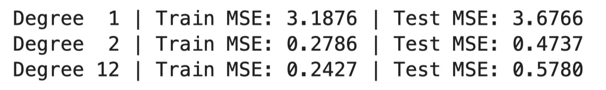

MSE ở các bậc khác nhau

Hoặc biểu diễn trực quan:

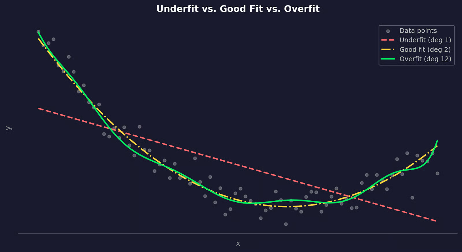
Dữ liệu được khớp với các bậc đa thức khác nhau

Bậc 1 cho lỗi cao trên cả hai tập - đó là thiếu khớp. Bậc 2 cân bằng tốt. Bậc 12 có lỗi huấn luyện thấp hơn nhưng lỗi kiểm thử cao hơn nhiều - đó là quá khớp.

Xác thực chéo

Cách đúng để tìm bậc tốt nhất là xác thực chéo - cụ thể là xác thực chéo k-phần.

Ý tưởng là chia dữ liệu của bạn thành k tập con, rồi huấn luyện trên k-1 tập và kiểm thử trên tập còn lại, lặp lại cho đến khi mỗi tập con đã được làm tập kiểm thử một lần. Cuối cùng, lấy trung bình lỗi trên tất cả các phần và làm vậy cho mỗi bậc ứng viên, rồi chọn bậc có lỗi kiểm thử trung bình thấp nhất.

Triển khai còn đơn giản hơn giải thích:

import numpy as np
from sklearn.preprocessing import PolynomialFeatures
from sklearn.linear_model import LinearRegression
from sklearn.model_selection import cross_val_score
from sklearn.pipeline import make_pipeline
import matplotlib.pyplot as plt

np.random.seed(42)

# Generate sample data
x = np.linspace(-3, 3, 80).reshape(-1, 1)
y = 0.6 * x.ravel()**2 - x.ravel() + np.random.normal(0, 0.6, 80)

# Test degrees 1 through 10
degrees = range(1, 11)
mean_errors = []

for deg in degrees:
    model = make_pipeline(PolynomialFeatures(deg), LinearRegression())
    scores = cross_val_score(model, x, y, cv=5, scoring="neg_mean_squared_error")
    mean_errors.append(-scores.mean())
    print(f"Degree {deg:>2} | Mean error: {-scores.mean():.4f}")

best_degree = np.argmin(mean_errors) + 1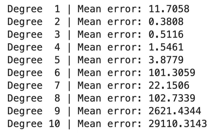

So sánh lỗi theo bậc

Hoặc biểu diễn trực quan:

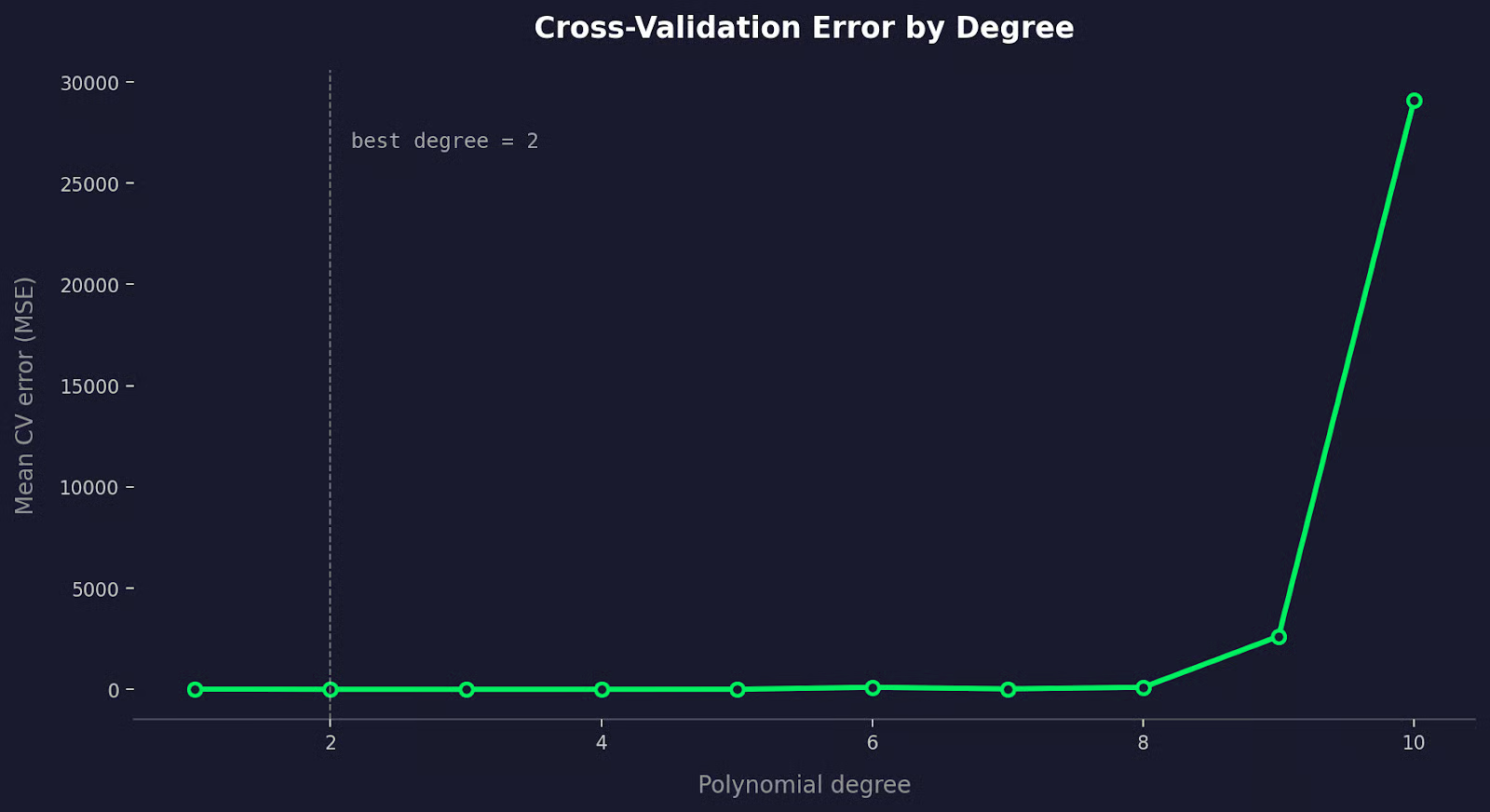
So sánh lỗi xác thực chéo

Lỗi CV giảm khi bạn thêm các hạng đa thức hữu ích, rồi tăng trở lại khi mô hình bắt đầu quá khớp.

Khi hai bậc cho lỗi CV tương tự, hãy chọn bậc thấp hơn. Một mô hình đơn giản đạt hiệu quả tương đương luôn là lựa chọn tốt hơn.

Những lưu ý và hạn chế chính

Có một vài cách mà hồi quy đa thức có thể dẫn bạn đến kết luận sai. Hãy cùng điểm qua.

Nhạy cảm với điểm ngoại lai

Điểm ngoại lai ảnh hưởng đến hồi quy đa thức nhiều hơn hồi quy tuyến tính.

Bình phương tối thiểu bình phương từng phần dư trước khi cộng dồn. Một điểm dữ liệu nằm xa xu hướng đóng góp một lỗi lớn không tương xứng, và mô hình sẽ bẻ cong đường để giảm lỗi đó - kể cả khi phải làm méo khớp ở mọi nơi khác.

Hiệu ứng này tệ hơn khi bậc tăng. Đa thức bậc cao đủ linh hoạt để đuổi theo một điểm ngoại lai, kéo đường cong rời xa phần lớn dữ liệu của bạn chỉ để khớp một điểm xấu.

Cách khắc phục là làm sạch dữ liệu trước khi khớp. Vẽ dữ liệu, xác định điểm ngoại lai, và quyết định liệu chúng là tín hiệu thực hay nhiễu. Nếu là nhiễu - lỗi đo lường, nhập liệu sai, bản ghi hỏng - hãy loại bỏ. Nếu là thật, cân nhắc phương pháp khớp ít nhạy với ngoại lai hơn như RANSAC hoặc hồi quy Huber.

Quá khớp

Mỗi lần bạn thêm một hạng đa thức, bạn cho mô hình thêm linh hoạt. Đến một điểm nào đó, sự linh hoạt đó không còn giúp ích, và mô hình bắt đầu khớp nhiễu ngẫu nhiên trong dữ liệu huấn luyện thay vì quy luật thực. Kết quả là một đường cong hoạt động tốt trên dữ liệu huấn luyện nhưng sụp đổ trên dữ liệu mới.

Điểm khó là quá khớp là vô hình nếu bạn chỉ nhìn vào lỗi huấn luyện. Một đa thức bậc 10 gần như luôn có MSE huấn luyện thấp hơn đa thức bậc 2. Điều đó không có nghĩa nó là mô hình tốt hơn.

Bạn nên tiếp cận như sau:

• Bắt đầu thấp: Thử bậc 2 hoặc 3 trước khi tăng cao hơn. Hầu hết các đường cong thực tế không cần quá mức đó
• Luôn đánh giá trên dữ liệu giữ lại: Lỗi huấn luyện không nói gì về khả năng khái quát hóa.
• Xác thực chéo: Dùng để tìm bậc mà lỗi kiểm thử ngừng cải thiện.
• Quan sát đường cong: Nếu đa thức của bạn làm điều gì đó "hoang dại" ngoài phạm vi dữ liệu huấn luyện, đó là dấu hiệu quá khớp.

Hồi quy đa thức hiệu quả nhất khi bạn có lý do xác đáng để kỳ vọng mối quan hệ cong, và bạn giữ được bậc đủ thấp.

Các lựa chọn thay thế cho hồi quy đa thức

Hồi quy đa thức không phải lúc nào cũng là công cụ phù hợp - một số phương án sau có thể hợp với bạn hơn.

Splines

Splines giải quyết vấn đề bất ổn toàn cục.

Khi bạn khớp một đa thức bậc 10, mọi hệ số đều bị ảnh hưởng bởi mọi điểm dữ liệu. Thay đổi ở một vùng của dữ liệu sẽ tác động đến đường cong ở khắp nơi. Splines tránh điều này bằng cách chia dữ liệu thành các đoạn và khớp một đa thức bậc thấp riêng cho từng đoạn. Các đoạn được nối tại các điểm gọi là nút (knots), với các ràng buộc giúp đường cong tổng thể mượt tại chỗ nối.

Kết quả là một đường cong linh hoạt ở nơi cần và ổn định ở nơi khác.

Trong Python, scipy và scikit-learn đều có các triển khai spline tốt:

from scipy.interpolate import UnivariateSpline

spline = UnivariateSpline(x, y, k=3)
y_pred = spline(x_new)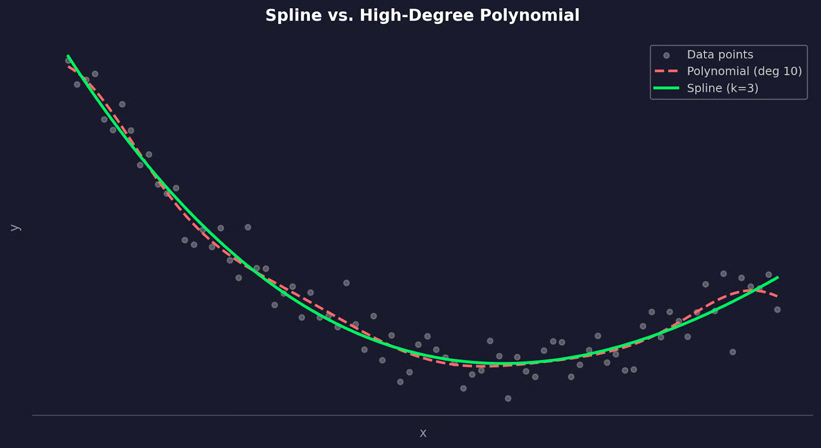

Spline so với đa thức bậc cao

Nhắc lại, hãy dùng splines khi dữ liệu của bạn có hành vi khác nhau ở các vùng khác nhau, hoặc khi một đường cong đa thức đơn lẻ không thể nắm bắt hình dạng nếu không tăng bậc quá cao.

Hồi quy véc-tơ hỗ trợ

Support Vector Regression (SVR) tiếp cận theo cách khác.

Nó không khớp một đường cong để tối thiểu hóa lỗi bình phương trên tất cả các điểm, mà cố tìm một hàm nằm trong biên độ sai số xác định đối với càng nhiều điểm càng tốt, đồng thời bỏ qua các điểm nằm trong biên đó. Điều này khiến nó ít nhạy với ngoại lai hơn hồi quy đa thức.

Kết nối với hồi quy đa thức đến từ thủ thuật kernel. SVR với kernel đa thức có thể khớp các mối quan hệ phi tuyến tương tự hồi quy đa thức - nhưng có khả năng khái quát hóa tốt hơn và kiểm soát nhiều hơn qua các tham số điều chuẩn.

from sklearn.svm import SVR

model = SVR(kernel="poly", degree=3, C=1.0, epsilon=0.1)
model.fit(x_train, y_train)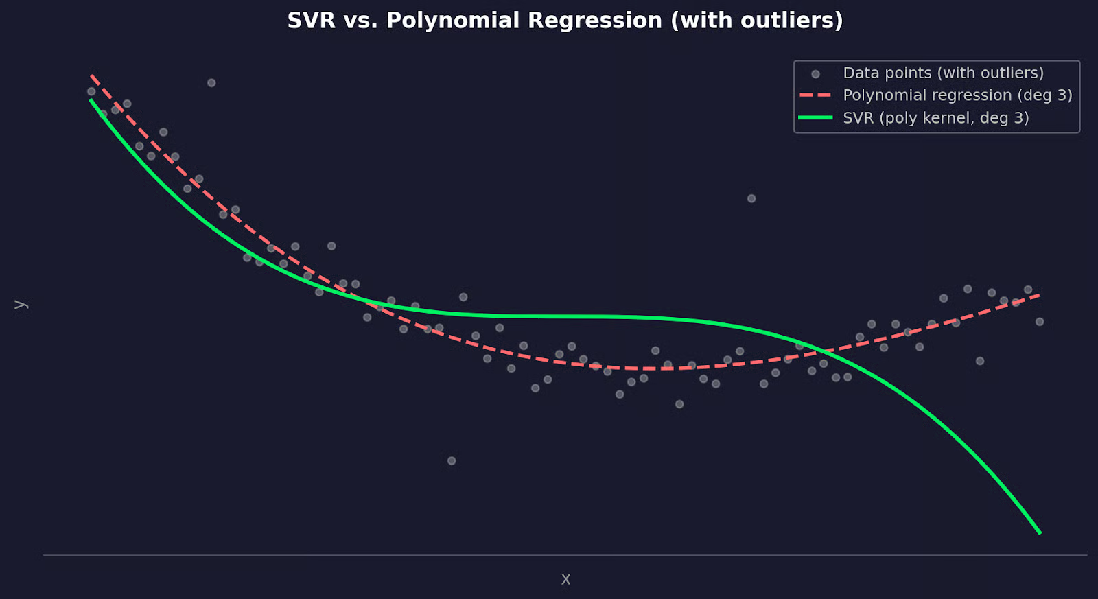

SVR so với đa thức bậc cao

SVR là lựa chọn tốt khi dữ liệu của bạn có ngoại lai mà bạn không thể loại bỏ, khi bạn cần kiểm soát tốt hơn điểm cân bằng giữa độ chệch và phương sai, hoặc khi hồi quy đa thức liên tục quá khớp dù đã xác thực chéo.

Kết luận

Trong bài viết này, tôi đã cho bạn thấy cách nó mở rộng hồi quy tuyến tính để khớp đường cong, cách ước lượng bình phương tối thiểu tìm ra các hệ số tốt nhất, và vì sao diễn giải từng hệ số riêng lẻ không nói lên nhiều điều.

Bậc bạn chọn quan trọng hơn bất cứ điều gì khác. Quá thấp dẫn đến thiếu khớp, quá cao dẫn đến quá khớp. Xác thực chéo mang đến cách khách quan để tìm điểm ngọt. Và nếu hồi quy đa thức không phù hợp, splines và SVR là những lựa chọn thay thế vững vàng đáng biết.

Cách tốt nhất để xây dựng trực giác cho tất cả những điều này là áp dụng trên dữ liệu của chính bạn. Chọn một bộ dữ liệu mà bạn nghi ngờ có mối quan hệ phi tuyến, khớp một mô hình tuyến tính trước, vẽ phần dư, và xem hồi quy đa thức làm khác đi như thế nào. Đọc hướng dẫn về Các mô hình phi tuyến và phân tích bằng R để xem pipeline này trong thực tế.