使用 Black Friday 数据集的机器学习教程

在本教程中，您将学习填充空值、预处理数据、使用 PCA 降维，以及使用 K-Fold 划分数据。

Rohit Peesa

已更新 2026年10月8日 · 10分钟阅读

使用 AI 探索

首先，让我们导入处理数据集所需的基础库。

import pandas as pd

现在读取数据集并查看它。

bfriday = pd.read_csv("BlackFriday.csv")

bfriday.head(10)

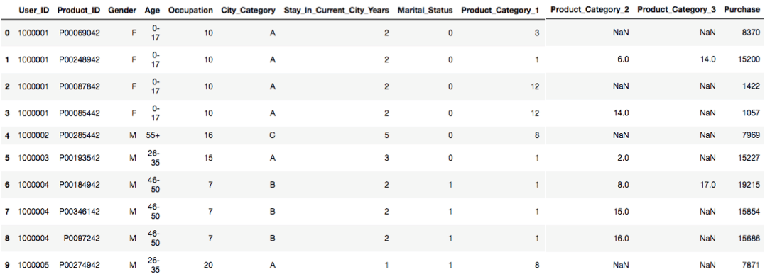
上述代码返回了包含 10 行（所有列）的数据集片段。如果您尝试使用 bfriday.head(x,y) 会报错，因为系统会默认要求提供全部列。bfriday.head() 也会给出输出，不会报错，且系统会自行选择返回的行和列。

bfriday.shape #this gives use dimensions of dataset(rows,columns)

(550068, 12)

bfriday['Stay_In_Current_City_Years'].value_counts()# counts the number of values per each range, bfriday['City_Category'].value_counts()

1    193821
2    101838
3     95285
5     84726
0     74398
Name: Stay_In_Current_City_Years, dtype: int64

bfriday.isnull().sum() #colculates no of null values for each category in dataset

User_ID                            0
Product_ID                         0
Gender                             0
Age                                0
Occupation                         0
City_Category                      0
Stay_In_Current_City_Years         0
Marital_Status                     0
Product_Category_1                 0
Product_Category_2            173638
Product_Category_3            383247
Purchase                           0
dtype: int64

b = ['Product_Category_2','Product_Category_3'] #here we are making an array consisting of 2 columns namely Product_Category_2,Product_Category_3

for i in b:
    exec("bfriday.%s.fillna(bfriday.%s.value_counts().idxmax(), inplace=True)" %(i,i))

现在我们用出现次数最多的值填充了空白。您也可以使用 bfriday.Product_Category_2.fillna(bfriday.Product_Category_2.value_counts().idxmax(),inplace=True) 来清理或填充空白，列 Product_Category_3 也可用同样的方法清理。

X = bfriday.drop(["Purchase"], axis=1)

我们从数据集中移除了名为 purchase 的列，并构建了名为 X 的数组，包含除 purchase 列外的所有列。

from sklearn.preprocessing import LabelEncoder#Now let's import encoder from sklearn library
LE = LabelEncoder()
#Now we will encode the data into labels using label encoder for easy computing

X = X.apply(LE.fit_transform)#Here we applied encoder onto data

现在我们将使用 pandas 把数据转换为数值形式，因为处理数值数据比处理类别型数据更容易。

X.Gender = pd.to_numeric(X.Gender)
X.Age = pd.to_numeric(X.Age)
X.Occupation = pd.to_numeric(X.Occupation)
X.City_Category = pd.to_numeric(X.City_Category)
X.Stay_In_Current_City_Years = pd.to_numeric(X.Stay_In_Current_City_Years)
X.Marital_Status = pd.to_numeric(X.Marital_Status)
X.Product_Category_1 = pd.to_numeric(X.Product_Category_1)
X.Product_Category_2 = pd.to_numeric(X.Product_Category_2)
X.Product_Category_3 = pd.to_numeric(X.Product_Category_3)

Y = bfriday["Purchase"]#Here we will made a array named as Y consisting of data from purchase column

from sklearn.preprocessing import StandardScaler
SS = StandardScaler()

通过去均值并缩放到单位方差来标准化特征。对每个特征的中心化与缩放相互独立，统计量在训练集样本上计算。随后会存储均值和标准差，以便在后续数据上通过 transform 方法使用。

Xs = SS.fit_transform(X)
#You must to transform X into numeric representation (not necessary binary).Because all machine learning methods operate on matrices of number

from sklearn.decomposition import PCA
pc = PCA(4)#here 4 indicates the number of components you want it into.

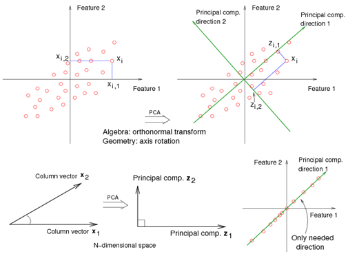
使用数据的奇异值分解进行线性降维，将其投影到低维空间。PCA 是最常用、最知名的降维方法之一。为了加速机器学习算法，您只对训练集拟合 PCA。主成分分析（PCA）。

PCA 用称为主成分的新变量替代原始变量，这些主成分之间协方差为零，且方差按降序排列。因此，来自数据的主成分之间的协方差矩阵呈对角形式。

来源：6.3 - Principal Components Analysis (PCA)

这里有个有趣的东西，叫做 RandomizedPCA

注意：切勿将 RandomizedPCA 用于稀疏数据。在稀疏数据上使用 RandomizedPCA 是不正确的，因为我们无法在不破坏稀疏性的情况下对数据进行中心化，这会在实际规模的稀疏数据上导致内存暴涨。然而，PCA 又要求进行中心化。

principalComponents = pc.fit_transform(X)#Here we are applying PCA to data/fitting data to PCA

pc.explained_variance_ratio_

array([7.35041374e-01, 2.64935995e-01, 1.10061180e-05, 6.21704987e-06])

principalDf = pd.DataFrame(data = principalComponents, columns = ["component 1", "component 2", "component 3", "component 4"])

from sklearn.model_selection import KFold
kf = KFold(20)
#Provides train/test indices to split data in train/test sets. Split dataset into k consecutive folds (without shuffling by default).
#Each fold is then used once as a validation while the k - 1 remaining folds form the training set.

for a,b in kf.split(principalDf):
    X_train, X_test = Xs[a],Xs[b]
    y_train, y_test = Y[a],Y[b]

from sklearn.linear_model import LinearRegression

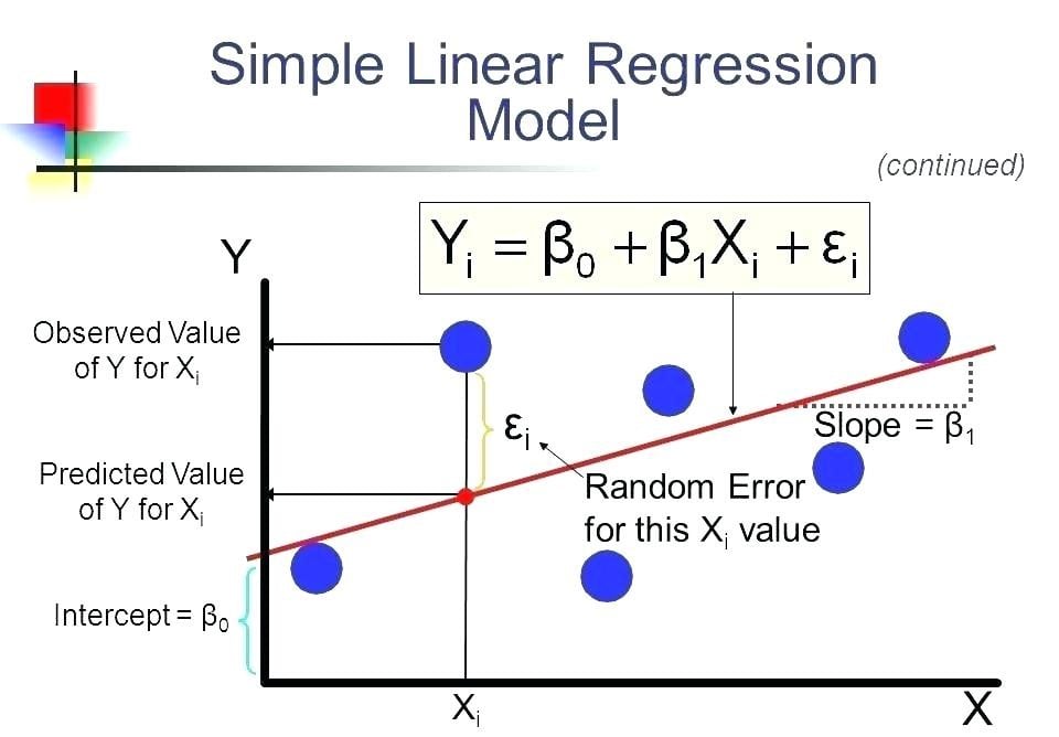
回归要研究两件事：(1) 一组自变量是否能很好地预测结果（因变量）？(2) 哪些变量是结果变量的重要预测因子，以及它们通过回归系数的大小与符号以何种方式影响结果？这些回归估计用于解释一个因变量与一个或多个自变量之间的关系。最简单的回归方程形式（一个因变量与一个自变量）由公式 y = c + b*x 定义，其中 y 为估计的因变量得分，c 为常数项，b 为回归系数，x 为自变量得分。

来源：Linear Regression

from sklearn.tree import DecisionTreeRegressor

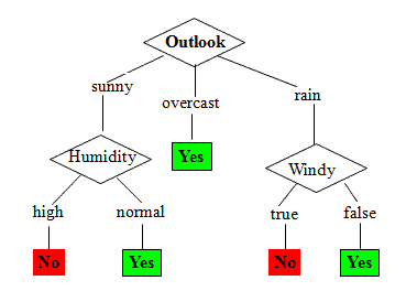
决策树自顶向下从根节点构建，通过将数据划分为包含相似取值实例的子集来进行建模。决策树以树结构的形式构建模型，它将数据集逐步划分为越来越小的子集，同时相应的决策树也逐步生成。最终的结果是一棵包含决策节点与叶节点的树。一个决策节点（如 Outlook）有两个或更多分支（如 Sunny、Overcast、Rainy），每个分支代表被测试属性的一个取值。叶节点（如 Hours Played）表示对数值目标的一个决策。树中最顶端的、对应最佳预测因子的决策节点称为根节点。决策树可以处理类别型与数值型数据。目标变量可取连续值（通常为实数）的决策树称为回归树。如果将树的最大深度设置得过高，决策树会学习训练数据中过于细微的细节甚至噪声，即发生过拟合。

来源：Decision Trees

from sklearn.ensemble import RandomForestRegressor

随机森林是一种估计器，它在数据集的不同子样本上拟合若干分类决策树，并通过平均化来提升预测精度、控制过拟合。若 bootstrap=True，则子样本通过有放回抽样生成，子样本大小与原始输入样本大小相同。该技术背后的思想是让多棵树去相关化。它在训练数据上生成不同的自助（bootstrap）样本，然后通过对树的结果求平均来降低方差。因此，这种方法会在 Python 或 R 中创建大量决策树。随机森林模型非常擅长处理带有数值特征的表格数据，或类别数少于数百的类别型特征。随机森林能够捕捉特征与目标之间的非线性交互。

注意：基于树的模型并不适用于非常稀疏的特征。当输入数据是稀疏的时，我们可以预处理稀疏特征以生成数值统计量，或者改用线性模型，这类模型更适合这种情形。

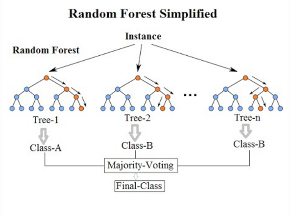
来源：Random Forest Simple Explanation by William Koehrsen

from sklearn.ensemble import GradientBoostingRegressor

梯度提升是一种用于回归与分类问题的机器学习技术，它以弱预测模型（通常是决策树）的集成为形式，构建预测模型。与其他提升方法类似，它以分阶段的方式构建模型，并通过允许对任意可微损失函数进行优化来加以推广。提升可被解释为对合适的代价函数进行优化的算法。后续的两篇论文将提升算法视为迭代的函数梯度下降算法。也就是说，这些算法在函数空间上优化代价函数，每次迭代选择一个沿负梯度方向前进的函数（弱假设）。这种函数梯度视角推动了提升算法在回归与分类之外的众多机器学习与统计领域的发展。梯度提升以迭代的方式将多个“弱学习器”组合为一个强学习器。用最小二乘回归的情境来解释最为直观：目标是通过最小化均方误差，令模型 F 学会预测 y ^ = F(x) 形式的值。

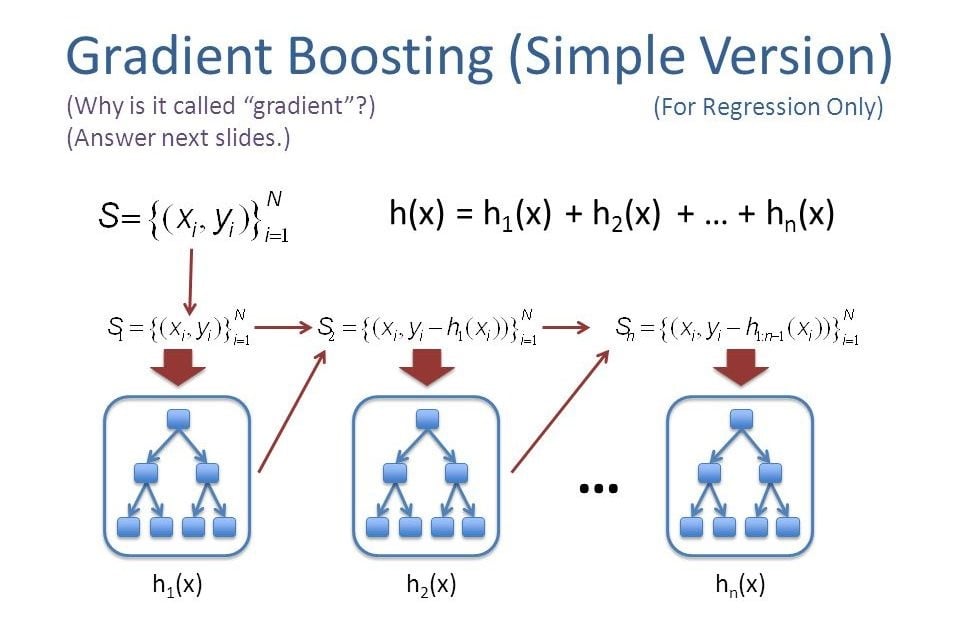
来源：Gradient Boosting Part1–Visual Conceptualization

lr = LinearRegression()
dtr = DecisionTreeRegressor()
rfr = RandomForestRegressor()
gbr = GradientBoostingRegressor()

fit1 = lr.fit(X_train,y_train)#Here we fit training data to linear regressor
fit2 = dtr.fit(X_train,y_train)#Here we fit training data to Decision Tree Regressor
fit3 = rfr.fit(X_train,y_train)#Here we fit training data to Random Forest Regressor
fit4 = gbr.fit(X_train,y_train)#Here we fit training data to Gradient Boosting Regressor

到目前为止您已经见过 fit 和 fit_transform，但可能还不清楚它们是什么？现在就来了解一下。

fit()：用于从训练数据中生成学习模型的参数。

transform()：将 fit() 方法生成的参数应用于模型，以产生变换后的数据集。

fit_transform()：在同一数据集上组合执行 fit() 与 transform() 接口。

print("Accuracy Score of Linear regression on train set",fit1.score(X_train,y_train)*100)
print("Accuracy Score of Decision Tree on train set",fit2.score(X_train,y_train)*100)
print("Accuracy Score of Random Forests on train set",fit3.score(X_train,y_train)*100)
print("Accuracy Score of Gradient Boosting on train set",fit4.score(X_train,y_train)*100)

Accuracy Score of Linear regression on train set 11.829233894211866
Accuracy Score of Decision Tree on train set 100.0
Accuracy Score of Random Forests on train set 94.207451077798
Accuracy Score of Gradient Boosting on train set 65.49517152859553

print("Accuracy Score of Linear regression on test set",fit1.score(X_test,y_test)*100)
print("Accuracy Score of Decision Tree on test set",fit2.score(X_test,y_test)*100)
print("Accuracy Score of Random Forests on test set",fit3.score(X_test,y_test)*100)
print("Accuracy Score of Gradient Boosting on testset",fit4.score(X_test,y_test)*100)

Accuracy Score of Linear regression on test set 36.8210287243639
Accuracy Score of Decision Tree on test set 57.61911563230391
Accuracy Score of Random Forests on test set 74.71675935214292
Accuracy Score of Gradient Boosting on testset 72.43849411693184