Machine Learning with Black Friday Dataset Tutorial

First let's import basic required library to deal with dataset.

import pandas as pd

Now let's read dataset and see it.

bfriday = pd.read_csv("BlackFriday.csv")

bfriday.head(10)

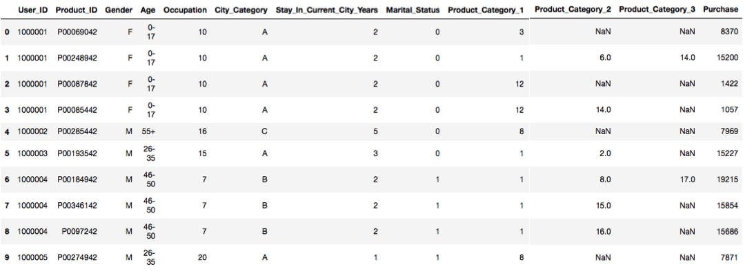
The above line gives us part of a dataset consisting of 10 rows and all columns. If you would try to give bfriday.head(x,y) it would be an error because computer already takes total no of columns mandatory.bfriday.head() this would also give you output and there won't be any error and computer takes both rows and columns of its choice

bfriday.shape #this gives use dimensions of dataset(rows,columns)

(550068, 12)

bfriday['Stay_In_Current_City_Years'].value_counts()# counts the number of values per each range, bfriday['City_Category'].value_counts()

1    193821
2    101838
3     95285
5     84726
0     74398
Name: Stay_In_Current_City_Years, dtype: int64

bfriday.isnull().sum() #colculates no of null values for each category in dataset

User_ID                            0
Product_ID                         0
Gender                             0
Age                                0
Occupation                         0
City_Category                      0
Stay_In_Current_City_Years         0
Marital_Status                     0
Product_Category_1                 0
Product_Category_2            173638
Product_Category_3            383247
Purchase                           0
dtype: int64

b = ['Product_Category_2','Product_Category_3'] #here we are making an array consisting of 2 columns namely Product_Category_2,Product_Category_3

for i in b:
    exec("bfriday.%s.fillna(bfriday.%s.value_counts().idxmax(), inplace=True)" %(i,i))

Now we will filled empty spaces with max value. We can also clean or fill empty spaces with bfriday.Product_Category_2.fillna(bfriday.Product_Category_2.value_counts().idxmax(),inplace=True) similarly you can clean column named Product_category_3

X = bfriday.drop(["Purchase"], axis=1)

We now removed column named purchase from the dataset and constructed an array named X which consists of all columns except a column of purchase.

from sklearn.preprocessing import LabelEncoder#Now let's import encoder from sklearn library
LE = LabelEncoder()
#Now we will encode the data into labels using label encoder for easy computing

X = X.apply(LE.fit_transform)#Here we applied encoder onto data

Now we will convert the data into the numerical form using pandas because dealing with numeric data would be easier than dealing with Categorical data

X.Gender = pd.to_numeric(X.Gender)
X.Age = pd.to_numeric(X.Age)
X.Occupation = pd.to_numeric(X.Occupation)
X.City_Category = pd.to_numeric(X.City_Category)
X.Stay_In_Current_City_Years = pd.to_numeric(X.Stay_In_Current_City_Years)
X.Marital_Status = pd.to_numeric(X.Marital_Status)
X.Product_Category_1 = pd.to_numeric(X.Product_Category_1)
X.Product_Category_2 = pd.to_numeric(X.Product_Category_2)
X.Product_Category_3 = pd.to_numeric(X.Product_Category_3)

Y = bfriday["Purchase"]#Here we will made a array named as Y consisting of data from purchase column

from sklearn.preprocessing import StandardScaler
SS = StandardScaler()

Standardize features by removing the mean and scaling to unit variance Centering and scaling happen independently on each feature by computing the relevant statistics on the samples in the training set. Mean and standard deviation are then stored to be used on later data using the transform method.

Xs = SS.fit_transform(X)
#You must to transform X into numeric representation (not necessary binary).Because all machine learning methods operate on matrices of number

from sklearn.decomposition import PCA
pc = PCA(4)#here 4 indicates the number of components you want it into.

Linear dimensionality reduction using Singular Value Decomposition of the data is to project it to a lower dimensional space.PCA is one of the most used and famous dimensionality reduction methods.PCA is for speeding up machine learning algorithms, you are fitting PCA on the training set only. Principal component analysis (PCA)

PCA replaces original variables with new variables, called principal components, which have zero covariations and have variances in decreasing order. So, the covariance matrix between the principal components extracted from the data.

We have something interesting here named as RandomizedPCA

Note:-Never use RandomizedPCA for sparse data.The use of RandomizedPCA on sparse data is incorrect as we cannot center the data without breaking the sparsity which can blow up the memory on realistically sized sparse data. However centering is required for PCA

principalComponents = pc.fit_transform(X)#Here we are applying PCA to data/fitting data to PCA

pc.explained_variance_ratio_

array([7.35041374e-01, 2.64935995e-01, 1.10061180e-05, 6.21704987e-06])

principalDf = pd.DataFrame(data = principalComponents, columns = ["component 1", "component 2", "component 3", "component 4"])

from sklearn.model_selection import KFold
kf = KFold(20)
#Provides train/test indices to split data in train/test sets. Split dataset into k consecutive folds (without shuffling by default).
#Each fold is then used once as a validation while the k - 1 remaining folds form the training set.

for a,b in kf.split(principalDf):
    X_train, X_test = Xs[a],Xs[b]
    y_train, y_test = Y[a],Y[b]

from sklearn.linear_model import LinearRegression

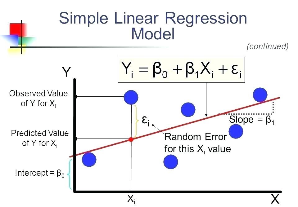
Regression is to examine two things: (1) does a set of predictor variables do a good job of predicting an outcome (dependent) variable? (2) Which variables, in particular, are significant predictors of the outcome variable, and in what way do they–indicated by the magnitude and sign of the beta estimates–impact the outcome variable? These regression estimates are used to explain the relationship between one dependent variable and one or more independent variables. The simplest form of the regression equation with one dependent and one independent variable is defined by the formula y = c + b*x, where y = estimated dependent variable score, c = constant, b = regression coefficient, and x = score on the independent variable.

from sklearn.tree import DecisionTreeRegressor

A decision tree is built top-down from a root node and involves partitioning the data into subsets that contain instances with similar values. Decision tree builds models in the form of a tree structure. It breaks down a dataset into smaller and smaller subsets while at the same time an associated decision tree is incrementally developed. The final result is a tree with decision nodes and leaf nodes. A decision node (e.g., Outlook) has two or more branches (e.g., Sunny, Overcast and Rainy), each representing values for the attribute tested. Leaf node (e.g., Hours Played) represents a decision on the numerical target. The topmost decision node in a tree which corresponds to the best predictor called root node. Decision trees can handle both categorical and numerical data. Decision trees where the target variable can take continuous values (typically real numbers) are called regression trees. If the maximum depth of the tree is set too high, the decision trees learn too fine details of the training data and learn from the noise, i.e. they overfit.

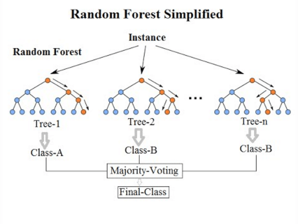
from sklearn.ensemble import RandomForestRegressor

A random forest is an estimator that fits a number of classifying decision trees on various sub-samples of the dataset and use averaging to improve the predictive accuracy and control over-fitting. The sub-sample size is always the same as the original input sample size but the samples are drawn with replacement if bootstrap=True. The idea behind this technique is to decorrelate the several trees. It generates on the different bootstrapped samples(i.e. self-generated samples) from training Data. And then we reduce the Variance in the Trees by averaging them. Hence, in this approach, it creates a large number of decision trees in python or R.The random forest model is very good at handling tabular data with numerical features, or categorical features with fewer than hundreds of categories. Random forests have the ability to capture the non-linear interaction between the features and the target.

Note:-Tree based models are not designed to work with very sparse features. When dealing with sparse input data, we can either pre-process the sparse features to generate numerical statistics or switch to a linear model, which is better suited for such scenarios.

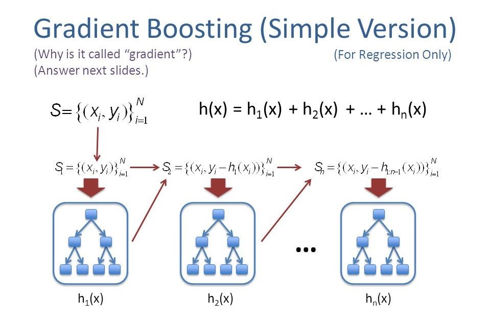
from sklearn.ensemble import GradientBoostingRegressor

Gradient boosting is a machine learning technique for regression and classification problems, which produces a prediction model in the form of an ensemble of weak prediction models, typically decision trees. It builds the model in a stage-wise fashion like other boosting methods do, and it generalizes them by allowing optimization of an arbitrary differentiable loss function. Boosting can be interpreted as an optimization algorithm on a suitable cost function. The latter two papers introduced the view of boosting algorithms as iterative functional gradient descent algorithms. That is, algorithms that optimize a cost function over function space by iteratively choosing a function (weak hypothesis) that points in the negative gradient direction. This functional gradient view of boosting has led to the development of boosting algorithms in many areas of machine learning and statistics beyond regression and classification.gradient boosting combines weak "learners" into a single strong learner in an iterative fashion. It is easiest to explain in the least-squares regression setting, where the goal is to "teach" a model F to predict values of the form y ^ = F ( x ) by minimizing the mean squared error.

lr = LinearRegression()
dtr = DecisionTreeRegressor()
rfr = RandomForestRegressor()
gbr = GradientBoostingRegressor()

fit1 = lr.fit(X_train,y_train)#Here we fit training data to linear regressor
fit2 = dtr.fit(X_train,y_train)#Here we fit training data to Decision Tree Regressor
fit3 = rfr.fit(X_train,y_train)#Here we fit training data to Random Forest Regressor
fit4 = gbr.fit(X_train,y_train)#Here we fit training data to Gradient Boosting Regressor

Till now you have seen fit and fit_transform but haven't understood what they are? Let's learn it now.

fit(): It is used for generating learning model parameters from training data

transform() :Parameters generated from fit() method,applied upon model to generate transformed data set.

fit_transform() :It is a combination of fit() and transform() api on same data set

print("Accuracy Score of Linear regression on train set",fit1.score(X_train,y_train)*100)
print("Accuracy Score of Decision Tree on train set",fit2.score(X_train,y_train)*100)
print("Accuracy Score of Random Forests on train set",fit3.score(X_train,y_train)*100)
print("Accuracy Score of Gradient Boosting on train set",fit4.score(X_train,y_train)*100)

Accuracy Score of Linear regression on train set 11.829233894211866
Accuracy Score of Decision Tree on train set 100.0
Accuracy Score of Random Forests on train set 94.207451077798
Accuracy Score of Gradient Boosting on train set 65.49517152859553

print("Accuracy Score of Linear regression on test set",fit1.score(X_test,y_test)*100)
print("Accuracy Score of Decision Tree on test set",fit2.score(X_test,y_test)*100)
print("Accuracy Score of Random Forests on test set",fit3.score(X_test,y_test)*100)
print("Accuracy Score of Gradient Boosting on testset",fit4.score(X_test,y_test)*100)

Accuracy Score of Linear regression on test set 36.8210287243639
Accuracy Score of Decision Tree on test set 57.61911563230391
Accuracy Score of Random Forests on test set 74.71675935214292
Accuracy Score of Gradient Boosting on testset 72.43849411693184

Conclusion

This tutorial provides a quick idea on how to fill null values. I wrote about it because most of the times real data is messier because you have nulls, wrong values and a lot of scraps which has to be cleaned. Hurray! You have completed this tutorial. If you any questions or thoughts on the tutorial, feel free to reach out in the comments below.

If you would like to learn more about Machine Learning in Python, check out DataCamp's Introduction to Machine Learning in Python tutorial and Preprocessing for Machine Learning in Python course.