SQL, also known as Structured Query Language, is a powerful tool to search through large amounts of data and return specific information for analysis. Learning SQL is crucial for anyone aspiring to be a data analyst, data engineer, or data scientist, and helpful in many other fields such as web development or marketing.
In this cheat sheet, you'll find a handy collection of information about window functions in SQL including what they are and how to construct them.
💻 To easily run all the example code in this tutorial yourself, you can create a DataLab workbook for free that has the dataset, SQL, and the code samples pre-configured. Great for experimenting!
Have this cheat sheet at your fingertips
Download PDFAssociate Data Engineer in SQL
Example dataset
We will use a dataset on the sales of bicycles as a sample. This dataset includes:
The [product] table
The product table contains the types of bicycles sold, their model year, and list price.
The [order] table
The order table contains the order_id and its date.
The [order_items] table
The order_items table lists the orders of a bicycle store. For each order_id, there are several products sold (product_id). Each product_id has a discount value.
What are Window Functions?
A window function makes a calculation across multiple rows that are related to the current row. For example, a window function allows you to calculate:
- Running totals (i.e. sum values from all the rows before the current row)
- 7-day moving averages (i.e. average values from 7 rows before the current row)
- Rankings
Similar to an aggregate function (GROUP BY), a window function performs the operation across multiple rows. Unlike an aggregate function, a window function does not group rows into one single row.
Syntax
Windows can be defined in the SELECT section of the query.
  SELECT
    window_function() OVER(
         PARTITION BY partition_expression
         ORDER BY order_expression
         window_frame_extent
    ) AS window_column_alias
    FROM table_name
To reuse the same window with several window functions, define a named window using the WINDOW keyword. This appears in the query after the HAVING section and before the ORDER BY section.
   SELECT
    window_function() OVER(window_name)
    FROM table_name
    [HAVING ...]
    WINDOW window_name AS (
         PARTITION BY partition_expression
         ORDER BY order_expression
         window_frame_extent
    )
    [ORDER BY ...]
Order by
ORDER BY is a subclause within the OVER clause. ORDER BY changes the basis on which the function assigns numbers to rows.
It is a must-have for window functions that assign sequences to rows, including RANK and ROW_NUMBER. For example, if we ORDER BY the expression price on an ascending order, then the lowest-priced item will have the lowest rank.
Let's compare the following two queries which differ only in the ORDER BY clause
   /* Rank price from LOW->HIGH */
   SELECT
       product_name,
       list_price,
       RANK() OVER
          (ORDER BY list_price ASC) rank
   FROM products

   /* Rank price from HIGH->LOW */
   SELECT
       product_name,
       list_price,
       RANK() OVER
          (ORDER BY list_price DESC) rank
   FROM products
Partition by
We can use PARTITION BY together with OVER to specify the column over which the aggregation is performed.
Comparing PARTITION BY with GROUP BY, we find the following similarity and difference:
Just like GROUP BY, the OVER subclause splits the rows into as many partitions as there are unique values in a column.
However, while the result of a GROUP BY aggregates all rows, the result of a window function using PARTITION BY aggregates each partition independently. Without the PARTITION BY clause, the result set is one single partition.
For example, using GROUP BY, we can calculate the average price of bicycles per model year using the following query.
  SELECT
   model_year,
   AVG(list_price) avg_price
FROM products
GROUP BY model_year
What if we want to compare each product’s price with the average price of that year? To do that, we use the AVG() window function and PARTITION BY the model year, as such.
   SELECT
   model_year,
   product_name,
   list_price,
   AVG(list_price) OVER
     (PARTITION BY model_year)
   avg_price
   FROM products
Notice how the avg_price of 2018 is exactly the same whether we use the PARTITION BY clause or the GROUP BY clause.
Window frame extent
A window frame is the selected set of rows in the partition over which aggregation will occur. Put simply, they are a set of rows that are somehow related to the current row.
A window frame is defined by a lower bound and an upper bound relative to the current row. The lowest possible bound is the first row, which is known as UNBOUNDED PRECEDING. The highest possible bound is the last row, which is known as UNBOUNDED FOLLOWING. For example, if we only want to get 5 rows before the current row, then we will specify the range using 5 PRECEDING.
Accompanying Material
You can use this https://bit.ly/3scZtOK to run any of the queries explained in this cheat sheet.
Ranking window functions
There are several window functions for assigning rankings to rows. Each of these functions requires an ORDER BY sub-clause within the OVER clause.
The following are the ranking window functions and their description:
|
Function Syntax |
Function Description |
Additional notes |
|
|
Assigns a sequential integer to each row within the partition of a result set. |
Row numbers are not repeated within each partition. |
|
|
Assigns a rank number to each row in a partition. |
|
|
|
Assigns the rank number of each row in a partition as a percentage. |
|
|
|
Distributes the rows of a partition into a specified number of buckets. |
|
|
|
The cumulative distribution: the percentage of rows less than or equal to the current row. |
|
We can use these functions to rank the product according to their prices.
   /* Rank all products by price */
SELECT
   product_name,
   list_price,
   ROW_NUMBER() OVER (ORDER BY list_price) AS row_num,
   DENSE_RANK() OVER (ORDER BY list_price) AS dense_rank,
   RANK() OVER (ORDER BY list_price) AS rank,
   PERCENT_RANK() OVER (ORDER BY list_price) AS pct_rank,
   NTILE(75) OVER (ORDER BY list_price) AS ntile,
   CUME_DIST() OVER (ORDER BY list_price) AS cume_dist
FROM products
Value window functions
FIRST_VALUE() and LAST_VALUE() retrieve the first and last value respectively from an ordered list of rows, where the order is defined by ORDER BY.
|
Value window function |
Function |
|
|
Returns the first value in an ordered set of values |
|
|
Returns the last value in an ordered set of values |
|
|
Returns the nth value in an ordered set of values. |
To compare the price of a particular bicycle model with the cheapest (or most expensive) alternative, we can use the FIRST_VALUE (or LAST_VALUE).
   /* Find the difference in price from the cheapest alternative */
SELECT
  product_name,
  list_price,
  FIRST_VALUE(list_price) OVER (
     ORDER BY list_price
     ROWS BETWEEN
         UNBOUNDED PRECEDING
         AND
         UNBOUNDED FOLLOWING
     ) AS cheapest_price,
FROM products
  /* Find the difference in price from the priciest alternative */
SELECT
   product_name,
   list_price,
   LAST_VALUE(list_price) OVER (
     ORDER BY list_price
     ROWS BETWEEN
        UNBOUNDED PRECEDING
        AND
        UNBOUNDED FOLLOWING
     ) AS highest_price
FROM products
Aggregate window functions
Aggregate functions available for GROUP BY, such as COUNT(), MIN(), MAX(), SUM(), and AVG() are also available as window functions.
|
Function Syntax |
Function Description |
|
|
Count the number of rows that have a non-null expression in the partition. |
|
|
Find the minimum of the expression in the partition. |
|
|
Find the maximum of the expression in the partition. |
|
|
Find the mean (average) of the expression in the partition. |
Suppose we want to find the average, maximum and minimum discount for each product, we can achieve it as such.
SELECT
   order_id,
   product_id,
   discount,
   AVG(discount) OVER (PARTITION BY product_id) AS avg_discount,
   MIN(discount) OVER (PARTITION BY product_id) AS min_discount,
   MAX(discount) OVER (PARTITION BY product_id) AS max_discount
FROM order_items
LEAD, LAG
The LEAD and LAG locate a row relative to the current row.
|
Function Syntax |
Function Description |
|
|
Accesses the value stored in a row after the current row. |
|
|
Accesses the value stored in a row before the current row. |
Both LEAD and LAG take three arguments:
Expression: the name of the column from which the value is retrievedOffset: the number of rows to skip. Defaults to 1.Default_value: the value to be returned if the value retrieved is null. Defaults toNULL.
With LAG and LEAD, you must specify ORDER BY in the OVER clause.
LEAD and LAG are most commonly used to find the value of a previous row or the next row. For example, they are useful for calculating the year-on-year increase of business metrics like revenue.
Here is an example of using lag to compare this year's sales to last year's.
   /* Find the number of orders in a year */
WITH yearly_orders AS (
   SELECT
	year(order_date) AS year,
	COUNT(DISTINCT order_id) AS num_orders
	FROM sales.orders
	GROUP BY year(order_date)
)

/* Compare this year's sales to last year's */
SELECT
   *,
   LAG(num_orders) OVER (ORDER BY year) last_year_order,
   LAG(num_orders) OVER (ORDER BY year) - num_orders diff_from_last_year
FROM yearly_orders
Similarly, we can make a comparison of each year's order with the next year's.
   /* Find the number of orders in a year */
WITH yearly_orders AS (
   SELECT
	year(order_date) AS year,
	COUNT(DISTINCT order_id) AS num_orders
	FROM sales.orders
	GROUP BY year(order_date)
)

/* Compare the number of years compared to next year */
SELECT *,
   LEAD(num_orders) OVER (ORDER BY year) next_year_order,
   LEAD(num_orders) OVER (ORDER BY year) - num_orders diff_from_next_year
FROM yearly_orders