Cours
Manipulation de données en SQL
4 h
324.1K
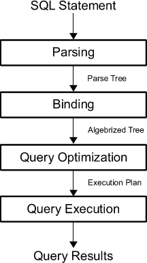
To improve the performance of your SQL query, you first have to know what happens internally when you press the shortcut to run the query.
First, the query is parsed into a “parse tree”; The query is analyzed to see if it satisfies the syntactical and semantical requirements. The parser creates an internal representation of the input query. This output is then passed on to the rewrite engine.
It is then the task of the optimizer to find the optimal execution or query plan for the given query. The execution plan defines exactly what algorithm is used for each operation, and how the execution of the operations is coordinated.
To indeed find the most optimal execution plan, the optimizer enumerates all possible execution plans, determines the quality or cost of each plan, takes information about the current database state, and then chooses the best one as the final execution plan. Because query optimizers can be imperfect, database users and administrators sometimes need to manually examine and tune the plans produced by the optimizer to get better performance.
Now you probably wonder what is considered to be a “good query plan.”
As you already read, the quality of the cost of a plan plays a considerable role. More specifically, things such as the number of disk I/Os that are required to evaluate the plan, the plan’s CPU cost and the overall response time that can be observed by the database client, and the total execution time are essential. That is where the notion of time complexity will come in. You’ll read more about this later on.
Next, the chosen query plan is executed, evaluated by the system’s execution engine, and the results of your query are returned.
What might not have become clear from the previous section is that the Garbage In, Garbage Out (GIGO) principle naturally surfaces within the query processing and execution: the one who formulates the query also holds the keys to the performance of your SQL queries. If the optimizer gets a poorly formulated query, it will only be able to do so much.
That means that there are some things that you can do when you’re writing a query. As you already saw in the introduction, the responsibility is two-fold: it’s not only about writing queries that live up to a certain standard, but also about gathering an idea of where performance problems might be lurking within your query.
An ideal starting point is to think of “spots” within your queries where issues might sneak in. And, in general, there are four clauses and keywords where newbies can expect performance issues to occur:
WHERE clause;INNER JOIN or LEFT JOIN keywords; And,HAVING clause;Granted, this approach is simple and naive, but as a beginner, these clauses and statements are excellent pointers, and it’s safe to say that when you’re just starting out, these spots are the ones where mistakes happen and, ironically enough, where they’re also hard to spot.
However, you should also realize that performance is something that needs context to become meaningful: merely saying that these clauses and keywords are bad isn’t the way to go when you’re thinking about SQL performance. Having a WHERE or HAVING clause in your query doesn’t necessarily mean that it’s a bad query.
Take a look at the following section to learn more about anti-patterns and alternative approaches to building up your SQL query. These tips and tricks are meant as a guide. How and if you actually need to rewrite your query depends on the amount of data, the database, and the number of times you need to execute the query, among other things. It entirely depends on the goal of your query, and having some prior knowledge about the database that you want to query is crucial!
The mindset of “the more data, the better” isn’t one that you should necessarily live by when you’re writing SQL queries: not only do you risk obscuring your insights by getting more than what you actually need, but also your performance might suffer from the fact that your query pulls up too much data.
That’s why it’s generally a good idea to look out for the SELECT statement, the DISTINCT clause and the LIKE operator.
SELECT StatementA first thing that you can already check when you have written your query is whether the SELECT statement is as compact as possible. Your aim here should be to remove unnecessary columns from SELECT. This way you force yourself only to pull up data that serves your query goal.
In case you have correlated subqueries that have EXISTS, you should try to use a constant in the SELECT statement of that subquery instead of selecting the value of an actual column. This is especially handy when you’re checking the existence only.
Remember that a correlated subquery is a subquery that uses values from the outer query. And note that, even though NULL can work in this context as a “constant”, it’s very confusing!
Consider the following example to understand what is meant by using a constant:
SELECT driverslicensenr, name FROM Drivers WHERE EXISTS (SELECT '1' FROM Fines WHERE fines.driverslicensenr = drivers.driverslicensenr);Tip: it’s handy to know that having a correlated subquery isn’t always a good idea. You can always consider getting rid of them by, for example, rewriting them with an INNER JOIN:
SELECT driverslicensenr, name FROM drivers INNER JOIN fines ON fines.driverslicensenr = drivers.driverslicensenr; DISTINCT ClauseThe SELECT DISTINCT statement is used to return only distinct (different) values. DISTINCT is a clause that you should definitely try to avoid if you can. As you have read in other examples, the execution time only increases if you add this clause to your query. It’s therefore always a good idea to consider whether you really need this DISTINCT operation to take place to get the results that you want to accomplish.
LIKE OperatorWhen you use the LIKE operator in a query, the index isn’t used if the pattern starts with % or _. It will prevent the database from using an index (if it exists). Of course, from another point of view, you could also argue that this type of query potentially leaves the door open to retrieve too many records that don’t necessarily satisfy your query goal.
Once again, your knowledge of the data that is stored in the database can help you to formulate a pattern that will filter correctly through all the data to find only the rows that really matter for your query.
When you cannot avoid filtering down your SELECT statement, you can consider limiting your results in other ways. Here’s where approaches such as the LIMIT clause and data type conversions come in.
TOP, LIMIT And ROWNUM ClausesYou can add the LIMIT or TOP clauses to your queries to set a maximum number of rows for the result set. Here are some examples:
SELECT TOP 3 * FROM Drivers;Note that you can further specify the PERCENT, for instance, if you change the first line of the query by SELECT TOP 50 PERCENT *.
SELECT driverslicensenr, name FROM Drivers LIMIT 2;Additionally, you can also add the ROWNUM clause, which is equivalent to using LIMIT in your query:
SELECT *FROM DriversWHERE driverslicensenr = 123456 AND ROWNUM <= 3;You should always use the most efficient, that is, smallest, data types possible. There’s always a risk when you provide a huge data type when a smaller one will be more sufficient.
However, when you add data type conversion to your query, you only increase the execution time.
An alternative is to avoid data type conversion as much as possible. Note also here that it’s not always possible to remove or omit the data type conversion from your queries, but that you should definitely aim to be careful in including them and that when you do, you test the effect of the addition before you run the query.
The data type conversions bring you to the next point: you should not over-engineer your queries. Try to keep them simple and efficient. This might seem too simple or stupid even to be a tip, mainly because queries can get complex.
However, you’ll see in the examples that are mentioned in the next sections that you can easily start making simple queries more complex than they need to be.
OR OperatorWhen you use the OR operator in your query, it’s likely that you’re not using an index.
Remember that an index is a data structure that improves the speed of the data retrieval in your database table, but it comes at a cost: there will be additional writes, and additional storage space is needed to maintain the index data structure. Indexes are used to quickly locate or look up data without having to search every row in a database every time the database table is accessed. Indexes can be created by using one or more columns in a database table.
If you don’t make use of the indexes that the database includes, your query will inevitably take longer to run. That’s why it’s best to look for alternatives to using the OR operator in your query;
Consider the following query:
SELECT driverslicensenr, nameFROM DriversWHERE driverslicensenr = 123456OR driverslicensenr = 678910OR driverslicensenr = 345678;You can replace the operator by:
IN; orSELECT driverslicensenr, nameFROM DriversWHERE driverslicensenr IN (123456, 678910, 345678);SELECT statements with a UNION.Tip: here, you need to be careful not to unnecessarily use the UNION operation because you go through the same table multiple times. At the same time, you have to realize that when you use a UNION in your query, the execution time will increase. Alternatives to the UNION operation are: reformulating the query in such a way that all conditions are placed in one SELECT instruction, or using an OUTER JOIN instead of UNION.
Tip: keep in mind also here that, even though OR -and also the other operators that will be mentioned in the following sections- likely isn’t using an index, index lookups aren’t always preferred!
NOT OperatorWhen your query contains the NOT operator, it’s likely that the index is not used, just like with the OR operator. This will inevitably slow down your query. If you don’t know what is meant here, consider the following query:
SELECT driverslicensenr, nameFROM DriversWHERE NOT (year > 1980);This query will definitely run slower than you would maybe expect, mainly because it’s formulated a lot more complex than it could be: in cases like this one, it’s best to look for an alternative. Consider replacing NOT by comparison operators, such as >, <> or !>; The example above might indeed be rewritten and become something like this:
SELECT driverslicensenr, nameFROM DriversWHERE year <= 1980;That already looks way neater, doesn’t it?
AND OperatorThe AND operator is another operator that doesn’t make use of the index, and that can slow your query down if used in an overly complex and inefficient way, like in the example below:
SELECT driverslicensenr, nameFROM DriversWHERE year >= 1960 AND year <= 1980;It’s better to rewrite this query and use BETWEEN operator:
SELECT driverslicensenr, nameFROM DriversWHERE year BETWEEN 1960 AND 1980;ANY and ALL OperatorsAlso, the ANY and ALL operators are some that you should be careful with because, by including these into your queries, the index won’t be used. Alternatives that will come in handy here are aggregation functions like MIN or MAX.
Tip: in cases where you make use of the proposed alternatives, you should be aware of the fact that all aggregation functions like SUM, AVG, MIN, MAX over many rows can result in a long-running query. In such cases, you can try to either minimize the number of rows to handle or pre-calculate these values. You see once again that it’s important to be aware of your environment, your query goal, … when you make decisions on which query to use!
Also in cases where a column is used in a calculation or in a scalar function, the index isn’t used. A possible solution would be to simply isolate the specific column so that it no longer is a part of the calculation or the function. Consider the following example:
SELECT driverslicensenr, nameFROM DriversWHERE year + 10 = 1980;This looks funky, huh? Instead, try to reconsider the calculation and rewrite the query to something like this:
SELECT driverslicensenr, nameFROM DriversWHERE year = 1970;This last tip means that you shouldn’t try to restrict the query too much because it can affect its performance. This is especially true for joins and for the HAVING clause.
When you join two tables, it can be important to consider the order of the tables in your join. If you notice that one table is considerably larger than the other one, you might want to rewrite your query so that the biggest table is placed last in the join.
When you add too many conditions to your joins, you obligate SQL to choose a particular path. It could be, though, that this path isn’t always the more performant one.
HAVING ClauseThe HAVING clause was initially added to SQL because the WHERE keyword could not be used with aggregate functions. HAVING is typically used with the GROUP BY clause to restrict the groups of returned rows to only those that meet certain conditions. However, if you use this clause in your query, the index is not used, which -as you already know- can result in a query that doesn’t really perform all that well.
If you’re looking for an alternative, consider using the WHERE clause. Consider the following queries:
SELECT state, COUNT(*) FROM Drivers WHERE state IN ('GA', 'TX') GROUP BY state ORDER BY stateSELECT state, COUNT(*) FROM Drivers GROUP BY stateHAVING state IN ('GA', 'TX') ORDER BY stateThe first query uses the WHERE clause to restrict the number of rows that need to be summed, whereas the second query sums up all the rows in the table and then uses HAVING to throw away the sums it calculated. In these types of cases, the alternative with the WHERE clause is obviously the better one, as you don’t waste any resources.
You see that this is not about limiting the result set, but instead about limiting the intermediate number of records within a query.
Note that the difference between these two clauses lies in the fact that the WHERE clause introduces a condition on individual rows, while the HAVING clause introduces a condition on aggregations or results of a selection where a single result, such as MIN, MAX, SUM,… has been produced from multiple rows.
You see, evaluating the quality, writing and rewriting of queries is not an easy job when you take into account that they need to be as performant as possible; Avoiding anti-patterns and considering alternatives will also be a part of responsibility when you write queries that you want to run on databases in a professional environment.
This list was just a small overview of some anti-patterns and tips that will hopefully help beginners; If you’d like to get an insight into what more senior developers consider the most frequent anti-patterns, check out this discussion.
What was implicit in the above anti-patterns is the fact that they actually boil down to the difference in set-based versus a procedural approach to building up your queries.
The procedural approach of querying is an approach that is much like programming: you tell the system what to do and how to do it.
An example of this is the redundant conditions in joins or cases where you abuse the HAVING clause, like in the above examples, in which you query the database by performing a function and then calling another function, or you use logic that contains loops, conditions, User Defined Functions (UDFs), cursors, … to get the final result. In this approach, you’ll often find yourself asking a subset of the data, then requesting another subset from the data and so on.
It’s no surprise that this approach is often called “step-by-step” or “row-by-row” querying.
The other approach is the set-based approach, where you just specify what to do. Your role consists of specifying the conditions or requirements for the result set that you want to obtain from the query. How your data is retrieved, you leave to the internal mechanisms that determine the implementation of the query: you let the database engine determine the best algorithms or processing logic to execute your query.
Since SQL is set-based, it’s hardly a surprise that this approach will be quite more effective than the procedural one and it also explains why, in some cases, SQL can work faster than code.
Tip the set-based approach of querying is also the one that most top employers in the data science industry will ask of you to master! You’ll often need to switch between these two types of approaches.
Note that if you ever find yourself with a procedural query, you should consider rewriting or refactoring it.
Knowing that anti-patterns aren’t static and evolve as you grow as an SQL developer and the fact that there’s a lot to consider when you’re thinking about alternatives also means that avoiding query anti-patterns and rewriting queries can be quite a difficult task. Any help can come in handy, and that’s why a more structured approach to optimize your query with some tools might be the way to go.
Note also that some of the anti-patterns mentioned in the last section had roots in performance concerns, such as the AND, OR and NOT operators and their lack of index usage. Thinking about performance doesn’t only require a more structured approach but also a more in-depth one.
Be however it may, this structured and in-depth approach will mostly be based on the query plan, which, as you remember, is the result of the query that’s first parsed into a “parse tree” and defines precisely what algorithm is used for each operation and how the execution of operations is coordinated.
As you have read in the introduction, it could be that you need to examine and tune the plans that are produced by the optimizer manually. In such cases, you will need to analyze your query again by looking at the query plan.
To get a hold of this plan, you will need to use the tools that your database management system provides to you. Some tools that you might have at your disposal are the following:
EXPLAIN PLAN statement in Oracle, but the name of the instruction varies according to the RDBMS that you’re working with. Elsewhere, you might find EXPLAIN (MySQL, PostgreSQL) or EXPLAIN QUERY PLAN (SQLite).Note that if you’re working with PostgreSQL, you make the difference between EXPLAIN, where you just get a description that states the idea of how the planner intends to execute the query without running it, while EXPLAIN ANALYZE actually executes the query and returns to you an analysis of the expected versus actual query plans. Generally speaking, a real execution plan is one where you actually run the query, whereas an estimated execution plan works out what it would do without executing the query. Although logically equivalent, an actual execution plan is much more useful as it contains additional details and statistics about what actually happened when executing the query.
In the remainder of this section, you’ll learn more about EXPLAIN and ANALYZE and how you can use these two to learn more about your query plan and the possible performance of your query. To do this, you’ll get started with some examples in which you’ll work with two tables: one_million and half_million.
You can retrieve the current information of the table one_million with the help of EXPLAIN; Make sure to put it right on top of your query, and when it’s run, it’ll give you back the query plan:
EXPLAINSELECT *FROM one_million;QUERY PLAN____________________________________________________Seq Scan on one_million(cost=0.00..18584.82 rows=1025082 width=36)(1 row)In this case, you see that the cost of the query is 0.00..18584.82 and that the number of rows is 1025082. The width of number of columns is then 36.
Also, you can then renew your statistical information with the help of ANALYZE.
ANALYZE one_million;EXPLAINSELECT *FROM one_million;QUERY PLAN____________________________________________________Seq Scan on one_million(cost=0.00..18334.00 rows=1000000 width=37)(1 row)Besides EXPLAIN and ANALYZE, you can also retrieve the actual execution time with the help of EXPLAIN ANALYZE:
EXPLAIN ANALYZESELECT *FROM one_million;QUERY PLAN___________________________________________________________Seq Scan on one_million(cost=0.00..18334.00 rows=1000000 width=37)(actual time=0.015..1207.019 rows=1000000 loops=1)Total runtime: 2320.146 ms(2 rows)The downside of using EXPLAIN ANALYZE here is obviously that the query is actually executed, so be careful with that!
Up until now, all the algorithms you have seen is the Seq Scan (Sequential Scan) or a Full Table Scan: this is a scan made on a database where each row of the table under scan is read in a sequential (serial) order, and the columns that are found are checked for whether they fulfill a condition or not. Concerning performance, the Sequential Scan is definitely not the best execution plan out there because you’re still doing a full table scan. However, it’s not too bad when the table doesn’t fit into memory: sequential reads go quite fast even with slow disks.
You’ll see more on this later on when you’re talking about the index scan.
However, there are some other algorithms out there. Take, for an example, this query plan for a join:
EXPLAIN ANALYZESELECT *FROM one_million JOIN half_millionON (one_million.counter=half_million.counter);QUERY PLAN_________________________________________________________________Hash Join (cost=15417.00..68831.00 rows=500000 width=42)(actual time=1241.471..5912.553 rows=500000 loops=1)Hash Cond: (one_million.counter = half_million.counter) -> Seq Scan on one_million (cost=0.00..18334.00 rows=1000000 width=37) (actual time=0.007..1254.027 rows=1000000 loops=1) -> Hash (cost=7213.00..7213.00 rows=500000 width=5) (actual time=1241.251..1241.251 rows=500000 loops=1) Buckets: 4096 Batches: 16 Memory Usage: 770kB -> Seq Scan on half_million (cost=0.00..7213.00 rows=500000 width=5)(actual time=0.008..601.128 rows=500000 loops=1)Total runtime: 6468.337 msYou see that the query optimizer chose for a Hash Join here! Remember this operation, as you’ll need this to estimate the time complexity of your query. For now, note that there is no index on half_million.counter, which you could add in the next example:
CREATE INDEX ON half_million(counter);EXPLAIN ANALYZESELECT *FROM one_million JOIN half_millionON (one_million.counter=half_million.counter);QUERY PLAN________________________________________________________________Merge Join (cost=4.12..37650.65 rows=500000 width=42)(actual time=0.033..3272.940 rows=500000 loops=1)Merge Cond: (one_million.counter = half_million.counter) -> Index Scan using one_million_counter_idx on one_million (cost=0.00..32129.34 rows=1000000 width=37) (actual time=0.011..694.466 rows=500001 loops=1) -> Index Scan using half_million_counter_idx on half_million (cost=0.00..14120.29 rows=500000 width=5)(actual time=0.010..683.674 rows=500000 loops=1)Total runtime: 3833.310 ms(5 rows)You see that, by creating the index, the query optimizer has now decided to go for a Merge join where Index Scans are happening.
Note the difference between the index scan and the full table scan or sequential scan: the former, which is also called “table scan”, scans the data or index pages to find the appropriate records, while the latter scans each row of the table.
You see that the total runtime has been reduced and the performance should be better, but there are two index scans, which makes that the memory will become more important here, especially if the table doesn’t fit into memory. In such cases, you first have to do a full index scan, which are fast sequential reads and pose no problem, but then you have a lot of random reads to fetch rows by index value. It’s those random reads that are generally orders of magnitude slower than sequential reads. In these cases, the full table scan is indeed faster than the full index scan.
Now that you have examined the query plan briefly, you can start digging deeper and think about the performance in more formal terms with the help of the computational complexity theory. This area in theoretical computer science that focuses on classifying computational problems according to their difficulty, among other things; These computational problems can be algorithms, but also queries.
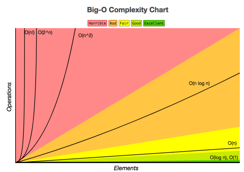
For queries, however, you’re not necessarily classifying them according to their difficulty, but rather to the time it takes to run it and get some results back. This is explicitly referred to as time complexity and to articulate or measure this type of complexity, you can use the big O notation.
With the big O notation, you express the runtime in terms of how quickly it grows relative to the input, as the input gets arbitrarily large. The big O notation excludes coefficients and lower order terms so that you can focus on the important part of your query’s running time: its rate of growth. When expressed this way, dropping coefficients and lower order terms, the time complexity is said to be described asymptotically. That means that the input size goes to infinity.
In database language, the complexity measures how much longer it takes a query to run as the size of the data tables, and therefore the database, increase.
Note that the size of your database doesn’t only increase as more data is stored in tables, but also the mere fact that indexes are present in the database also plays a role in the size.
As you have seen before, the execution plan defines, among other things, what algorithm is used for each operation, which makes that every query execution time can be logically expressed as a function of the table size involved in the query plan, which is referred to as a complexity function. In other words, you can use the big O notation and your execution plan to estimate the query complexity and the performance.
In the following subsections, you’ll get a general idea about the four types of time complexities, and you’ll see some examples of how queries’ time complexity can vary according to the context in which you run it.
Hint: the indexes are part of the story here!
Note, though, that there are different types of indexes, different execution plans and different implementations for various databases to consider, so that the time complexities listed below are very general and can vary according to your specific setting.
An algorithm is said to run in constant time if it requires the same amount of time regardless of the input size. When you’re talking about a query, it will run in constant time if it requires the same amount of time irrespective of the table size.
These type of queries are not really common, yet here’s one such an example:
SELECT TOP 1 t.* FROM tThe time complexity is constant because you select one arbitrary row from the table. Therefore, the length of the time should be independent of the size of the table.
An algorithm is said to run in linear time if its time execution is directly proportional to the input size, i.e. time grows linearly as input size increases. For databases, this means that the time execution would be directly proportional to the table size: as the number of rows in the table grows, the time for the query grows.
An example is a query with a WHERE clause on a un-indexed column: a full table scan or Seq Scan will be needed, which will result in a time complexity of O(n). This means that every row needs to be read to find the one with the right ID. You don’t have a limit at all, so every row does need to be read, even if the first row matches the condition.
Consider also the following example of a query that would have a complexity of O(n) if there’s no index on i_id:
SELECT i_id FROM item;COUNT(*) FROM TABLE; will have a time complexity of O(n), because a full table scan will be required unless the total row count is stored for the table. Then, the complexity would be more like O(1).Closely related to the linear execution time is the execution time for execution plans that have joins in them. Here are some examples:
Remember: a nested join is a join that compares every record in one table against every record in the other.
An algorithm is said to run in logarithmic time if its time execution is proportional to the logarithm of the input size; For queries, this means that they will run if the execution time is proportional to the logarithm of the database size.
This logarithmic time complexity is true for query plans where an Index Scan or clustered index scan is performed. A clustered index is an index where the leaf level of the index contains the actual data rows of the table. A clustered is much like any other index: it is defined on one or more columns. These form the index key. The clustering key is then the key columns of a clustered index. A clustered index scan is then basically the operation of your RDBMS reading through for the row or rows from top to bottom in the clustered index.
Consider the following query example, where the there’s an index on i_id and which would generally result in a complexity of O(log(n)):
SELECT i_stock FROM item WHERE i_id = N; Note that without the index, the time complexity would have been O(n).
An algorithm is said to run in quadratic time if its time execution is proportional to the square of the input size. Once again, for databases, this means that the execution time for a query is proportional to the square of the database size.
A possible example of a query with quadratic time complexity is the following one:
SELECT * FROM item, author WHERE item.i_a_id=author.a_id The minimum complexity would be O(n log(n)), but the maximum complexity could be O(n^2), based on the index information of the join attributes.
To summarize, you can also look at the following cheat sheet to estimate the performance of queries according to their time complexity and how well they would be performing:
With the query plan and the time complexity in mind, you can consider tuning your SQL query further. You could start by paying particular attention to the following points:
Congrats! You have made it to the end of this blog post, which just gave you a small peek at SQL query performance. You hopefully got more insights into anti-patterns, the query optimizer, and the tools you can use to review, estimate and interpret the complexity of your query plan. There is, however, much more to discover! If you want to know more, consider reading the book “Database Management Systems”, written by R. Ramakrishnan and J. Gehrke.
Finally, I don’t want to withhold you this quote from a StackOverflow user:
“My favorite antipattern is not testing your queries.
This applies when:
- Your query involves more than one table.
- You think you have an optimal design for a query, but don’t bother to test your assumptions.
- You accept the first query that works, with no clue about whether it’s even close to optimized."
If you want to get started with SQL, consider taking these DataCamp courses:
Learn more about SQL
Cours
cheat-sheet
Richie Cotton
Tutoriel
Sejal Jaiswal
Tutoriel
Sayak Paul
Tutoriel
Sayak Paul
code-along
Kelsey McNeillie
code-along
Adel Nehme