The Julia programming language is a scientific computing language that was first announced in 2012. Since then, Julia has become a serious contender in the data programming language landscape. With its ease of use, speed, and support for scientific computing use cases, learning Julia is a viable path for many data scientists today.
This article provides an in-depth and lengthy tutorial on the Julia programming language for beginners, covering basic syntax, working with different data types, vectors and strings, data frames, and much more.
Why learn Julia?
There are many reasons behind Julia’s rise to popularity. While Python and R reign supreme as the most widely used programming languages in data science, Julia has been downloaded over 35 million times. The reasons behind its growth are thoroughly outlined in this article, but here’s a summary of Julia’s features and advantages:
- Speed: One of Julia’s main founding principles is that it needs to be as general as Python, as statistics-friendly as R, but as fast as C. This enables faster data workflows, especially for scientific computing.
- Syntax: Another way Julia shines is its syntax. Despite its speed, Julia’s syntax is dynamically-typed, making it closer to R and Python than more complex programming languages. This means it's much more accessible and easy to learn than other high-performance programming languages.
- Multiple dispatch: Without getting too technical, another advantage of Julia is multiple dispatch, which refers to Julia functions’ ability to behave differently based on the types of arguments it is given. This makes it a flexible language to work with.
Because of these features, Julia was in the top 5 of most loved languages in the 2022 StackOverflow developer survey. This is especially the case for folks in the scientific community who are looking to transition from tools such as Matlab.
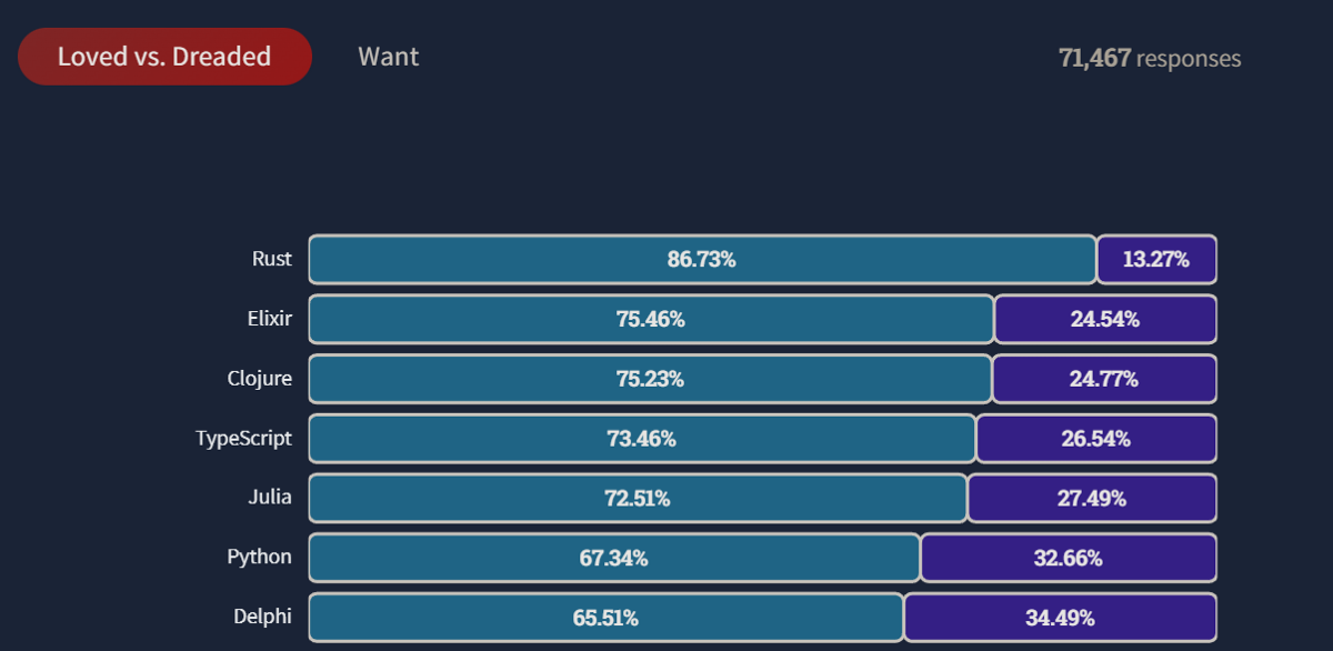
Screenshot from the StackOverflow Developer Survey 2022
With that out of the way, let’s dive deep into how to get started with Julia.
How to install and run Julia?
Installing Julia is straightforward. Download the installer specific to your operating system on this page of the Julia website and check the box that adds Julia to the system PATH. If you type julia in the command line and get the following output, everything is running OK.
Installing and running the Julia programming language
Both PyCharm and VSCode offer Julia plugins that support code highlighting and debugging. However, since data scientists usually like to work within JupyterLab, it’s also easy to add a Julia kernel to JupyterLab. After entering the julia prompt in the terminal, simply enter these two lines:
using Pkg
add("IJulia")
The code adds the IJulia package to the Julia installation on the system. Restart any running JupyterLab sessions, and you should see the Julia option in the Launcher.
Julia running in JupyterLab
Basic Julia syntax
This section will cover the fundamentals of Julia syntax, including variables, data types, operators, vectors, and so on.
Operators
In programming, there are special characters called operators that represent specific mathematical or logical processes. Below you will see the most common operators, including addition, subtraction, multiplication, subtraction, and more.
Note: In Julia, comments are written with single # characters. Anything written after the # gets ignored by the program (till the end of the line).
# Addition in Julia
37 + 73110# Subtraction in Julia
17 - 19-2# Multiplication in Julia
29 * 33957# Division in Julia
22 / 73.142857142857143# Backwards division in Julia, the above is equal to 0 / 5.
5 \ 00# The remainder operator in Julia
98456 % 23
16# Raising to the power 2 (squaring)
(22 / 7) ^ 29.877551020408163# Raising to the power 3 (cubing)
-7 ^ 3-343# Raising to the power 0.5 (square-rooting)
(355 / 133) ^ 0.51.633760365638372Variables
In programming, we use variables to store information. Variables make it easy to refer to a piece of information via a name. For example, here we’re storing the number 73 into a variable called a, and the string “Hello world!” in the variable “word” (we’ll look at Julia's different data types in the following section). Typing the name of the variable at the command line prints its value.
# Storing the number 73 in a variable a
a = 73
a73# Storing "Hello world!" in word
word = "Hello world!"
wordHello world!All Julia operators and functions work the same on variables.
# Multiplying two numeric variables
a = 73
b = 37
a * b2701You can use any alphanumeric character in variable names, including underscores. However, there are certain conventions in naming them in Julia. Variable names:
- are
lower_snake_case(lowercase and words are separated by an underscore) - cannot start with a number.
Introduction to data types in Julia
Data types tell the program what values a variable takes and what kind of mathematical or logical operators can be used on them without causing an error. There are various data types in Julia, below you can find the most basic ones.
|
Data type |
Expression |
Examples |
Description |
|
Integers |
|
1, -99 |
Whole numbers |
|
Floats |
|
1.23, 4.0 |
Numbers with a decimal point |
|
Booleans |
|
true, false |
Logical values |
|
Strings |
|
"Hello", "A", "" |
Text data with any number of characters |
|
Characters |
|
'A', '$', '\u20AC' |
Text data with exactly one character |
The data type of a variable can be printed using the typeof() function:
# Getting the type of 3.14
typeof(3.14)Float64When performing operations in Julia, you need to be mindful of the consequences of different data types. For example, multiplying a float and an integer returns a float.
# Bank balance as an integer
balance = 100

# Interest rate as a float
interest_rate = 1.05

# Interest rate as a float
new_balance = balance * interest_rate

typeof(new_balance)Float64Conversely, performing operations on strings and numeric data types often leads to an error. Such as the following.
# Bank balance as an integer
balance = 100

# Interest rate as a string
interest_rate = “5%”

# Interest rate as a float
new_balance = balance * interest_rate
ERROR: MethodError:
no method matching *(::Int64, ::String)Converting data types in Julia
It is possible to convert different data types into other data types in Julia with dedicated functions that come out of the box. Below is a table containing how to convert different data types in Julia.
|
From |
To |
Function |
|
Integer |
Float |
|
|
Float |
Integer |
|
|
Integer or float |
String |
|
|
String |
Float |
|
|
String |
Integer |
|
Working with characters and strings in Julia
We saw the character and string data types in Julia in the previous section, in this section, we’ll dive deep into common character and string operations. As a reminder, a string is an ordered series of characters or plain-old text inside double quotes.
# A string is a series of characters
word = "Hello world!"
word
"Hello world!"To write a multi-line string, you can use triple quotes:
multi_line = """
   This is a
   multi-line string.
"""
print(multi_line)
This is a
multi-line string.You can extract information and attributes from strings in a variety of ways. For example, bracket indexing can extract individual characters or a range of characters based on their position. In this example, 1:3 denotes the sequence of numbers from 1 to 3 inclusive.
text = "Julia is a high-level, dynamic programming language"
# Extracting the first character in text based on its index
text[1]
'J': ASCII/Unicode U+004A (category Lu: Letter, uppercase)# Extracting the first three characters in text based on its index
text[1:3]"Jul"Above we put 1 inside the brackets, and it returned the first character. Alternatively, you can also use the special begin operator:
# Extracting the first character in text with the begin operator
text[begin]
'J': ASCII/Unicode U+004A (category Lu: Letter, uppercase)When you extract a single character from a string, it will have a Char data type.
# Extract the type of the fourth character
typeof(text[4])Char# Extract the type of the fourth character
typeof(text[4])However, when you slice a string and extract more than one character, the output is a string as well.
# Extract the type of the first 5 characters
typeof(text[begin:5])StringAbove, we are slicing the first five characters of text. Keep in mind that both indices on either side of the colon are inclusive. Unlike Python, negative indices are not supported. Instead, you will use the end operator with a negative number. For example, to get the third character from the end of the string, you can write the following.
# Third from the end of the string
text[end-2]
'a': ASCII/Unicode U+0067 (category Ll: Letter, lowercase)Common string operations in Julia
You can use the length() function to count the number of characters in a string.
# Count the number of characters in a string
length(text)51A common task is to combine two or more strings together. You can accomplish this with the string() function, passing strings into the function separated by commas.
# Creating one string from "Julia", "is", "awesome"
string("Julia ", "is ", "awesome!")
"Julia is awesome!"You can also use the * (multiplication) operator to combine strings together
# Creating one string by multiplying strings
"73 " * "is " * "the " * "best " * "prime."
"73 is the best prime."In both ways, remember to leave a space between the words. Another way of joining strings is by repeating a string multiple times. Here is how it is done with ^ (exponentiation) operator:
# Creating one string with the exponentiation operator
"Three times the fun!" ^ 3
"Three times the fun! Three times the fun! Three times the fun!"Arrays in Julia
Another common data type in Julia and other languages are arrays, as they are called in Julia. Arrays are a list of values stored in between brackets []. Arrays are called differently based on their dimensions.
- One-dimensional arrays are called vectors.
- Two-dimensional arrays are called matrices.
- Three-dimensional arrays and above are just called arrays.
In this tutorial, we will focus exclusively on vectors. Vectors can be created by passing items into a pair of brackets, as seen below.
# Define a three-integer vector
x = [1, 2, 3]
3-element Vector{Int64}:
1
2
3# Get the type of x
typeof(x)Vector{Int64} (alias for Array{Int64, 1})The vector x has the Vector type, which is an alias for a one-dimensional array (as listed by the output alias for Array{In664, 1}). All its elements have Int64 data type. But that does not always mean all elements must have the same type. For example, here’s a vector with elements of different types.
# Define a vector with various data types
array = [1, "Hello", 22/7]
3-element Vector{Any}:
1
"Hello"
3.142857142857143As you can see, the vector elements have the Any data type inside the curly braces, which represent multiple data types. You can even pass vectors into vectors.
# Define a vector with various data types, including another vector
array = [1, 2, 3, ["Hello", 73]]
4-element Array{Any,1}:
1
2
3
Any["Hello", 73]The length() function works the same on vectors as strings, as it counts the number of elements inside the array.
# Get the length of a vector
length(array)3Indexing rules work similarly as well — here, we’re indexing the first and second elements in the array.
# Get the first element of a vector
array = [1, "Hello", 22/7]
array[begin]1# Get the last element of a vector
array[end-1]"Hello"Boolean operators and numeric comparisons
Programming languages use Boolean values to implement logic. A Boolean can only have two values: true or false. Boolean values are especially useful when working with numeric comparisons and Boolean operators. Let’s first look at numeric comparisons.
Numeric comparison operators in Julia
In the table below, you’ll find the most commonly used numeric comparison operators in Julia. As you’ll see in the examples, you can compare Booleans, numeric objects, and more using numeric comparison operators. Notice that you can use one or two symbols to write less/greater than or equal to. To use the one symbol version, type \le then TAB or \ge then TAB.
|
Operator |
Name |
Example |
|
|
equality |
|
|
|
inequality |
|
|
|
less than |
|
|
|
less than or equal to |
|
|
|
greater than |
|
|
|
greater than or equal to |
|
Boolean operators in Julia
Outside of numeric comparison operators, there are Boolean operators — such as and/or. They can be used to combine two or more Boolean expressions into one. Below you’ll find the most common Boolean operators and how they’re used.
|
Operator |
Name |
Examples |
|
|
and operator |
|
|
|
or operator |
|
Intermediate Julia syntax
Conditional statements in Julia
Using Boolean values and operators, you can write conditional statements. For example, if something evaluates to true — perform an operation. If false, perform another. Conditional statements are also called if/else statements. Here is how they are written:
if true
   print("Do something")
else
   print("Do something else")
end
Whenever a condition after the if keyword evaluates to true, the if block is executed, otherwise, the else block is executed. This example shows a conditional that checks if a number is even or odd.
number = 5

if number % 2 == 0
   print("The number is even")
else
   print("The number is odd")
end
The number is oddIn the expression after if, we are using the modulus operator, %, to check if the number returns 0 as a remainder when divided by 2. It evaluates to false because the remainder of dividing 5 by 2 is 1. Therefore, the else clause is executed. Now, let’s use our knowledge of Boolean operators and conditional statements to write a program that checks if a number is positive, negative, or zero.
number = 0

if number > 0
   print("The number is positive.")
elseif number == 0
   print("The number is equal to zero.")
else
   print("The number is negative.")

end
The number is equal to zero.We are adding the new condition using the elseif clause. We use elseif clauses when we have to check for two or more conditions in exact order.
For loops
A for loop in programming is used to iterate and perform operations on each element of a sequence (string, vector, tuple, set, etc.) in order. The for-loop syntax is straightforward in Julia. For example, let’s build a loop that prints each element of a vector:
languages = ["Julia", "Python", "R"]

for lang = languages
   println(lang)

end
Julia
Python
RThe for loop is started by writing the for keyword. Then, we choose a temporary variable name. In this case, we are choosing lang, whose value changes as we go through the vector languages. Then, to specify we are looping through languages, we write its name after the assignment operator =.
Inside the loop, we use the println() function to print each element of languages, represented by the lang temporary variable. lang is called a temporary variable because it is not accessible once the loop finishes.
Note: The difference between print() and println() is that println() prints items on new lines.
You can use everything you’ve learned up to this point inside for loops. For example, let’s create an array of 10 integers and only print odd numbers in it:
integers_vector = [1, 2, 3, 4, 5, 6, 7, 8, 9, 10]

for i = integers_vector
   # Print only odd numbers
   if i % 2 == 1
       println(i)
   end
end
1
3
5
7
9Don’t forget to close both the for loop and the if statement with end.
You can also iterate through strings as well since they are also sequences. Here, for example, we are printing each letter in the string "Julia".
for letter = "Julia"
   println(letter)

end
J
u
l
i
aInstalling packages in Julia
All the operators (+, -, *, ^), functions (print(), println(), typeof()) and keywords (for, if, else) we have been using come with the Julia installation. However, the code in the installation is not enough to solve all of our problems. We need to install packages to load tools and functions for extra functionality. Packages are libraries of pre-written code (by other programmers) that we can add to our Julia installation, which help us solve specific problems.
For example, we will install two packages called DataFrames and CSV which help us manipulate information in CSV files. Here is how to do it:
using Pkg
Pkg.add("DataFrames")
Pkg.add("CSV")
The Pkg class is a global Julia package manager. Its add() function adds new packages to the installation. To import all the function names from the libraries, we import them with the using keyword at the top of our scripts.
using DataFrames
using CSV
We will use their functions in the next section.
Getting started with DataFrames
A DataFrame is a special data type in data science languages like Julia, Python, or R designed to work with tables. The most popular file format for storing tables is a CSV (comma-separated values). The DataFrame library will have the tools to load such files and manipulate the information within.
Importing CSV files
We will be importing the diamonds dataset for this tutorial. The diamonds.csv file looks like this:
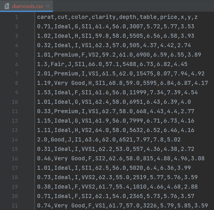
Access the diamonds dataset here
The first line is called the header and contains the column names. Let’s load it using the CSV and DataFrames packages.
# Load in the diamonds DataFrame
diamonds = DataFrame(CSV.File("data/diamonds.csv"))
typeof(diamonds)DataFrameWe pass the path to the CSV file to CSV.File(), which in turn, is passed into the DataFrame() function. The output of typeof() shows the operation was successful.
Simple data manipulation
The first thing you always do when you have a new DataFrame is to print a few rows of it to see what it looks like. You can do that with the first() function.
# Print the first 7 rows of diamond
first(diamonds, 7)
7 × 10 DataFrame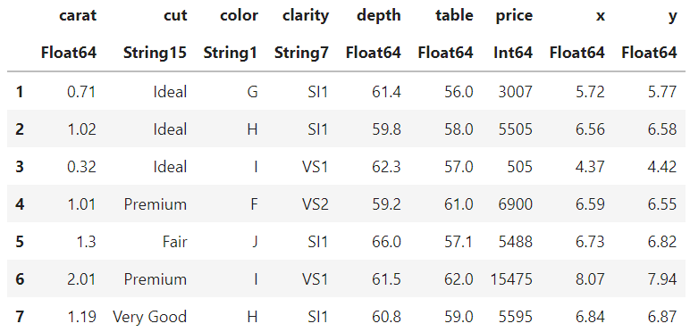
First 7 rows of the diamonds dataset
The first() function returns the first n-rows of a DataFrame. As we can see, there are 6 numeric and 3 categorical (text) columns. The index is also counted as a column in Julia DataFrames.
There is also the last() function that works similarly to first(). You can already guess what it does from the name. Yup, it gets the last n rows.
Another useful function is size(). It prints the number of rows and columns of a DataFrame.
# Print the dimensions of diamonds
size(diamonds)
(10000, 10)The one we have has 10 thousand rows and 10 columns (including the index). The naked eye cannot handle all 10k rows, so we use summary statistics to get a feel of the distribution of the columns in our dataset. To do that, we use the describe() function
# Summary statistics of diamonds using describe()
describe(diamonds)
10 × 7 DataFrame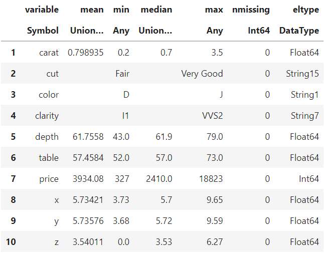
Output of the describe() function
The output is a summary table with 7 columns. The min, max, mean, and median columns only apply to numeric columns. In the eltype column, you can see the data types of each column in diamonds. The numbers next to String refer to the length of the longest string in that column.
You can also use the following syntax to select individual columns from the DataFrame.
# Extracting the first 10 rows of the cut column
diamonds[:, :cut][begin:10]
10-element PooledArrays.PooledArray{String15,UInt32,1,Array{UInt32,1}}:
"Ideal"
"Ideal"
"Ideal"
"Premium"
"Fair"
"Premium"
"Very Good"
"Ideal"
"Ideal"
"Premium"The first colon inside the brackets selects all the rows. Then, we specify the column name after a comma and another colon (no quotes). Then, we use indexing on the returned array to select the first ten rows. To make the above code, even simpler, we could select the first ten rows directly inside the first brackets like below:
# Extracting the first 10 rows of the cut column
diamonds[1:10, :carat]
10-element PooledArrays.PooledArray{String15,UInt32,1,Array{UInt32,1}}:
"Ideal"
"Ideal"
"Ideal"
"Premium"
"Fair"
"Premium"
"Very Good"
"Ideal"
"Ideal"
"Premium"To select multiple columns, put the column names (combined with a colon) inside brackets.
# Extracting the first 5 rows of the cut, carat, price columns
diamonds[1:5, [:carat, :cut, :price]]
5 × 3 DataFrame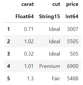
The first 5 rows and 3 columns of the diamonds dataset
Let’s run the describe() function only on the numeric columns
# Running describe on numeric columns only
describe(diamonds[:, [:carat, :depth, :table, :price, :x, :y]])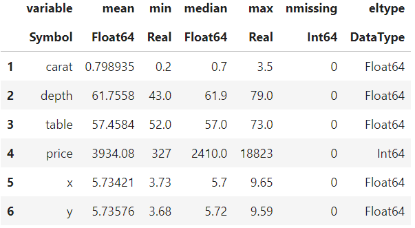
Running describe() on numeric columns only
To see the DataFrame sorted in ascending order based on a column, use the sort() function:
# Sort diamonds and see the first 5 rows
sorted_diamonds = sort(diamonds, :price)
first(sorted_diamonds, 5)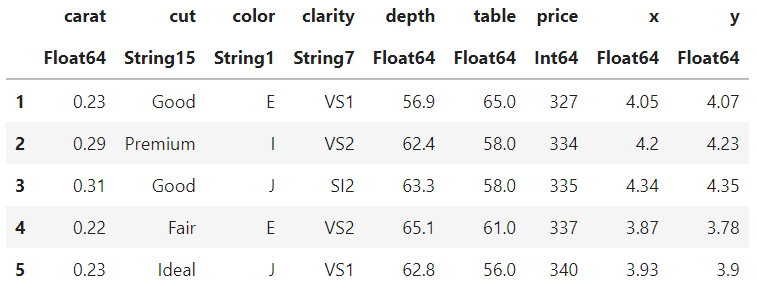
The sorted summary table
To sort in descending order, wrap the order() function around the column name.
# Sort diamonds in descending order and see the first 5 rows
sorted_diamonds = sort(diamonds, order(:price, rev=true))
first(sorted_diamonds, 5)
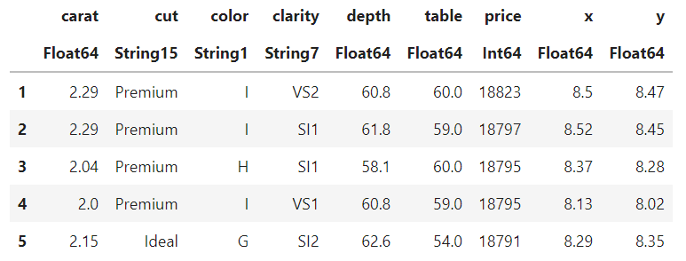
The sorted summary table, descending
Awesome! Now, you can load DataFrames and perform basic data exploration.
Learn more about Julia
Even though Julia is a young programming language, there is already a wealth of resources to master the language. Here are some of them to boost your skills:
- The rise of Julia — Is it worth learning in 2022?
- Progressing from MATLAB to Julia
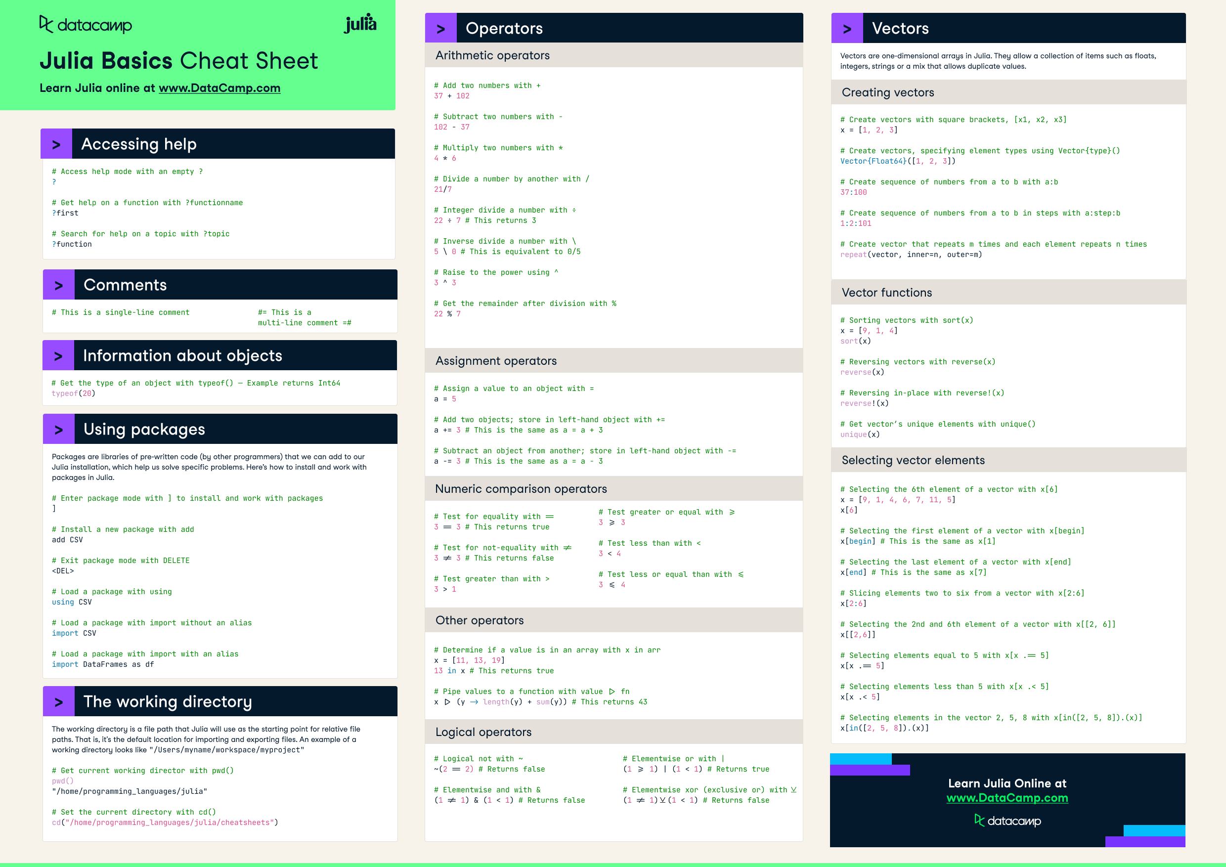
- Check out our cheat sheets, covering all data tools and technologies, including Julia
- Check out our Introduction to Julia course