
Course
MLOps Concepts
2 hr
42.6K

Have you ever looked back on a machine learning project and wondered why you made specific decisions, or even what the code is actually doing? For example, why did you choose this subset of features, which version of data did you train the final model on, or how did different sets of model hyperparameters affect performance? Sounds like you need to adopt experimentation best practices into your machine learning projects!
Machine learning experimentation is the process of designing, building, logging, and evaluating a machine learning pipeline to identify the model that achieves a desired performance in terms of a given metric or metrics, e.g., F1 score, RMSE, etc. It is a crucial step in developing machine learning models both prior to deployment and as part of retraining. Just like any other experiment, it should be designed to:
By keeping these goals in mind you can ensure you can easily find what you need, such as a model's hyperparameters or a version of a dataset, and share information, such as model performance and source code.
Luckily, this is where Weights & Biases comes in!
Weights & Biases is a platform and Python library for machine learning engineers to run experiments, log artifacts, automate hyperparameter tuning, and evaluate performance. This tutorial will introduce the core functionality by demonstrating a machine learning pipeline where the key elements are logged and subsequently examined in a dashboard!
# Install Python library
!pip install wandb
To login, you'll need to sign up for an account.
Once created, visit the authorize page to access an API key that you can use to login. Make a note of this, but don't share it with anyone else!
To login, either open a new Terminal and enter wandb login or add a new cell to your notebook and execute !wandb login.
You will be prompted to provide your API key, which you can copy and paste, to successfully login. Your credentials will be stored locally in ~/.netrc going forward.
wandb loginWeights & Biases has several components including Experiments, Artifacts, Sweeps, and Models. Let's start by looking at the core of the workflow - creating and running experiments.
# Import required modules
import pandas as pd
import numpy as np
import seaborn as sns
import matplotlib.pyplot as plt
import wandb
from sklearn.model_selection import train_test_split, GridSearchCV, KFold
from sklearn.linear_model import LinearRegression, Ridge
from sklearn.tree import DecisionTreeRegressor
from sklearn.metrics import mean_squared_error, r2_score
In Weights & Biases an Experiment is also known as a project. To create a new project we call the wand.init() function, pass our project name as a string to the project keyword argument. You can assign this to a variable called run, so we can log important files, models, and metrics, to the run.
Optionally, you can also provide a string to the job_type keyword argument, allowing you to easily distinguish between different steps such EDA, feature engineering, or hyperparameter tuning. Additionally, the code you execute can be logged by setting save_code equal to True.
# Initialize a run
run = wandb.init(project="predicting_london_temperature",
                 job_type="Baseline modeling",
save_code=True)You can log any important information, such as datasets, variables, or files, as an Artifact. To do this, first create a variable by calling wandb.Artifact(), providing the name and type. Then log this using the wandb.log_artifact() function. Let's start by logging the original dataset.
original_data = "london_weather.csv"
# Create an Artifact
data_artifact = wandb.Artifact(name="original_dataset",
                               type="data",
                               description="London weather dataset")
# Add the file to the Artifact
data_artifact.add_file(original_data)
# Log the Artifact as part of the run
run.log_artifact(data_artifact)
Exploratory Data Analysis (EDA) is a crucial step in the machine learning workflow, helping you to ensure data conforms to required data types and is free from missing values and outliers. It is also an opportunity to examine distributions and relationships between features.
The added benefit of using Weights & Biases is that we can log the data as we perform preprocessing, along with any visualizations produced.
# Read in the data
london = pd.read_csv(original_data)

# Previewing the first five rows
london.head()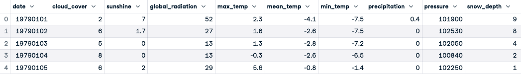
# Visualize distributions
plt.figure(figsize=(12,8))
london.hist()
plt.tight_layout()
plt.show()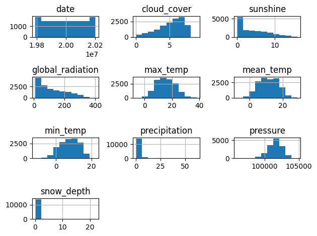
# View data types and non-null counts
london.info()


<class 'pandas.core.frame.DataFrame'>
RangeIndex: 15341 entries, 0 to 15340
Data columns (total 10 columns):
 #   Column            Non-Null Count  Dtype
---  ------            --------------  -----
 0   date              15341 non-null  int64
 1   cloud_cover       15322 non-null  float64
 2   sunshine          15341 non-null  float64
 3   global_radiation  15322 non-null  float64
 4   max_temp          15335 non-null  float64
 5   mean_temp         15305 non-null  float64
 6   min_temp          15339 non-null  float64
 7   precipitation     15335 non-null  float64
 8   pressure          15337 non-null  float64
 9   snow_depth        13900 non-null  float64
dtypes: float64(9), int64(1)
memory usage: 1.2 MB


# Convert date to datetime
london["date"] = pd.to_datetime(london["date"], format="%Y%m%d")

# Add a month column
london["month"] = london["date"].dt.month

# Drop missing values
london.dropna(inplace=True)
Now the data has been cleaned, you can log it as an Artifact using wand.Artifact().
# Save and log the new version of the data
london.to_csv("london_weather_preprocessed.csv", index=False)
preprocessed_data = "london_weather_preprocessed.csv"
# Create an Artifact
preprocessed_data_artifact = wandb.Artifact(name="london_weather_preprocessed",
                               type="data",
                               description="London weather dataset - preprocessed")
# Add the file to the Artifact
preprocessed_data_artifact.add_file(preprocessed_data)
# Log the Artifact as part of the run
run.log_artifact(preprocessed_data_artifact)


<wandb.sdk.artifacts.local_artifact.Artifact at 0x15bfe6710>The next step in the workflow is to identify potential features for modeling while avoiding multicollinearity. To do this, you can first produce a correlation heatmap, then use Ridge Regression to quantify feature importance in predicting "mean_temperature".
# Correlation heatmap
sns.heatmap(london.corr(), annot=True, center=True)
plt.show()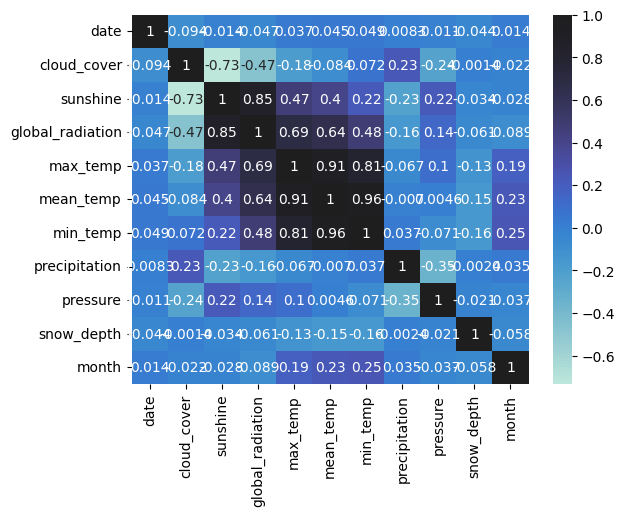
You can log this plot using wandb.Image()!
# Log the heatmap
wandb.log({"correlation_heatmap": wandb.Image(plt)})


# Split the data
X = london.drop(columns=["mean_temp", "min_temp", "max_temp", "date"])
y = london["mean_temp"]
X_train, X_test, y_train, y_test = train_test_split(X, y, random_state=42, test_size=0.2)

# Build a Ridge regression model
ridge = Ridge(alpha=0.1)
ridge.fit(X_train, y_train)
y_pred = ridge.predict(X_test)

# Visualize feature importance using the coefficients
fig = plt.figure()
sns.barplot(x=X_train.columns, y=ridge.coef_)
plt.xticks(rotation=30)
plt.tight_layout()
plt.savefig("feature_selection.png")
plt.show()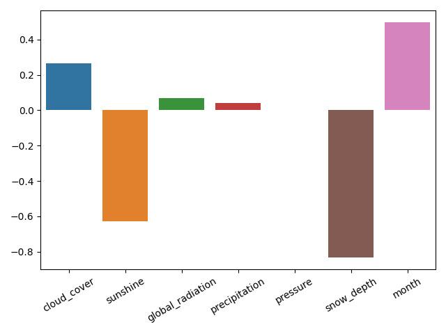
Let's save the model and feature importance plot using pickle.dump() and wandb.log().
import pickle
pickle.dump(ridge, open("feature_selection_model.pkl", "wb"))
feature_selection_model = wandb.Artifact("feature_selection_model", type="model")
feature_selection_model.add_file("feature_selection_model.pkl")
run.log_artifact(feature_selection_model)
wandb.log({"feature_selection_plot": wandb.Image(fig)})


<Figure size 640x480 with 0 Axes>You made it! Time to train your baseline model using the identified important features, which are any with a Ridge model coefficient of more than zero. You'll also log the new training and test data.
X = london[["cloud_cover", "global_radiation", "precipitation", "month"]]
y = london["mean_temp"]
X_train, X_test, y_train, y_test = train_test_split(X, y, random_state=42, test_size=0.2)

def log_data(X_train, y_train, X_test, y_test):
    # Log the training and test data
    training_features = wandb.Artifact(name="X_train",
                               type="data",
                               description="Training features")
    X_train.to_csv("X_train.csv", index=False)
    training_features.add_file("X_train.csv")
    run.log_artifact(training_features)

    training_labels = wandb.Artifact(name="y_train",
                               type="data",
                               description="Training labels")
    y_train.to_csv("y_train.csv", index=False)

    training_labels.add_file("y_train.csv")
    run.log_artifact(training_labels)

    test_features = wandb.Artifact(name="X_test",
                               type="data",
                               description="Test features")
    X_test.to_csv("X_test.csv", index=False)
    test_features.add_file("X_test.csv")
    run.log_artifact(test_features)

    test_labels = wandb.Artifact(name="y_test",
                               type="data",
                               description="Test labels")
    y_test.to_csv("y_test.csv", index=False)
    test_labels.add_file("y_test.csv")
    run.log_artifact(test_labels)

log_data(X_train, y_train, X_test, y_test)
Let's train and evaluate a Decision Tree Regression model, using Root Mean Squared Error (RMSE) and R-Squared as performance metrics.
# Fit and evaluate the model
dt_reg = DecisionTreeRegressor(random_state=42)
dt_reg.fit(X_train, y_train)
y_pred = dt_reg.predict(X_test)
rmse = mean_squared_error(y_test, y_pred, squared=False)
r_squared = r2_score(y_test, y_pred)
print(rmse, r_squared)


3.8627385194713346 0.5399282872125385

# Save and log the model and metrics
pickle.dump(dt_reg, open("baseline_decision_tree.pkl", "wb"))
baseline_model = wandb.Artifact("baseline_decision_tree", type="model")
baseline_model.add_file("baseline_decision_tree.pkl")
run.log_artifact(baseline_model)
wandb.log({"rmse": rmse, "r_squared": r_squared})
You can drill down further on model performance by visualizing the model's residuals. Weights & Biases has a function in their sklearn module to produce this!
# Plot training residuals
wandb.log({"baseline_residuals_plot": wandb.sklearn.plot_residuals(dt_reg, X_train, y_train)})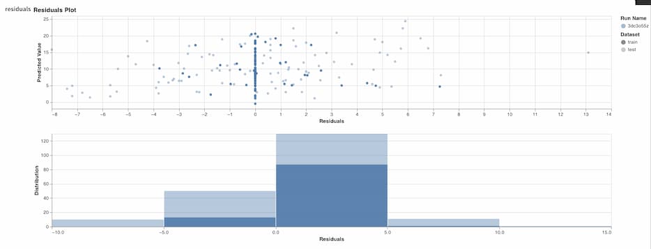
Training and evaluation is complete, so let's finish the current run.
# Finish run
wandb.finish()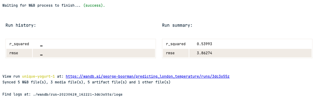
Now you've created and logged a baseline model with its associated performance metrics, let’s look at how you can perform hyperparameter tuning and version your models using Weights & Biases and scikit-learn.
We'll use GridSearchCV to search for the best performing model across a hyperparameter space, based on RMSE.
# Initialize a new run
run_v2 = wandb.init(project="predicting_london_temperature",
job_type="Hyperparameter tuning",
save_code=True)
# Split the data and create a KFold object
X_train, X_test, y_train, y_test = train_test_split(X, y, random_state=42, test_size=0.2)
kf = KFold(n_splits=5, shuffle=True, random_state=42)
# Create the hyperparameter space
params = {"max_depth":[2, 5, 8, 12, 20],
"min_samples_split": [2, 5, 8, 12, 20],
"max_features": [1, 2, 3, 4],
"random_state": [42]
}
# Create a GridSearchCV object
dt_reg = DecisionTreeRegressor()
dt_reg_cv = GridSearchCV(dt_reg,
params,
cv=kf,
scoring="neg_root_mean_squared_error")
# Fit the data
dt_reg_cv.fit(X_train, y_train)
# Evaluate and log performance
## GridSearchCV uses negative RMSE
## so you can convert it to positive
print(f"Best RMSE: {-1 * dt_reg_cv.best_score_})")
print(f"Best model: {dt_reg_cv.best_estimator_}")
# Save and log the model, metrics, and parameters
pickle.dump(dt_reg_cv, open("tuned_decision_tree.pkl", "wb"))
tuned_decision_tree = wandb.Artifact("tuned_decision_tree", type="model")
tuned_decision_tree.add_file("tuned_decision_tree.pkl")
run_v2.log_artifact(tuned_decision_tree)
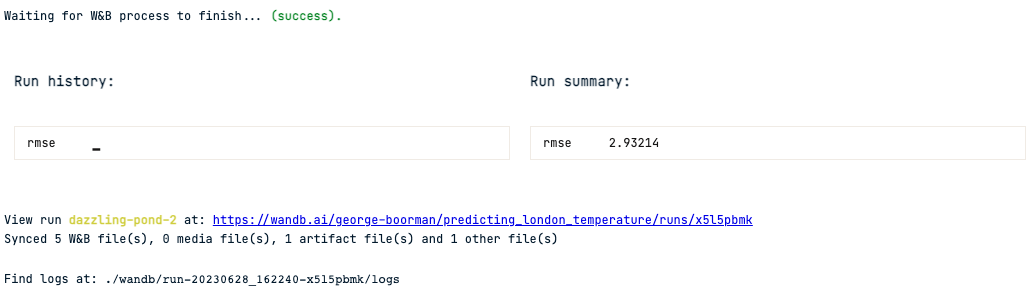
wandb.log({"rmse": -1 * dt_reg_cv.best_score_})
wandb.finish()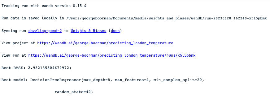
To examine runs and artifacts you can go to www.wandb.ai/<your-profile-name>/projects then select the project you have created.
Once inside, you will see each run that you've created, along with any media, such as plots, like this:
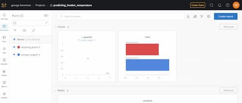
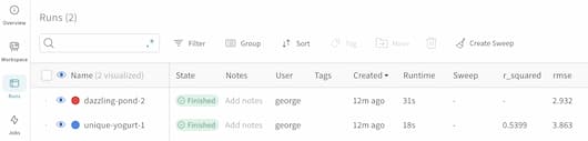
By clicking on the Runs icon, you can see all your runs and key information, including metrics logged like RMSE and R-Squared.
Weights & Biases has a lot more functionality that you can explore, such as using existing artifacts as part of new runs, a Command Line Interface tool, and Prompts for the development of LLMs!
To reinforce your knowledge about machine learning experimentation and the wider techniques of MLOps, you might want to check out:
Learn topics mentioned in this tutorial!
Course
Course
Course
blog
Nisha Arya Ahmed
12 min
blog
DataRobot Inc
6 min
Tutorial
Joanne Xiong
Tutorial
Amberle McKee
code-along
Jinen Setpal
code-along
Folkert Stijnman