Curso
More than a year ago, we launched DataCamp Workspace, our cloud-based notebook IDE, designed to enable practitioners and teams to seamlessly work with data and collaborate online. As of today, thousands of individuals and teams use Workspace to analyze data and share their insights, build portfolio projects, and compete in competitions.
We recently migrated our RStudio workspaces to DataCamp’s Notebook Editor or JupyterLab. This means R users can enjoy the latest Workspace features, including sharing, collaborating, commenting, native SQL integration, and more. In this blog post, we outline the key features of JupyterLab, how it differs from RStudio, and how R users can take advantage of the DataCamp Notebook Editor.

JupyterLab: A Next-Generation Notebook Interface
JupyterLab is a web-based interactive development environment for R and Python notebooks, alongside other programming languages. Designed specifically for data science and machine learning workflows, its rich interface consists of a notebook, terminal, text editor, and file browser. Its modular design also invites the open-source community to create extensions for expanding JupyterLab’s functionality. In JupyterLab, the output of each cell of code appears once a cell is run. Like in an R Markdown notebook, users can also intersperse code blocks with markdown annotations.
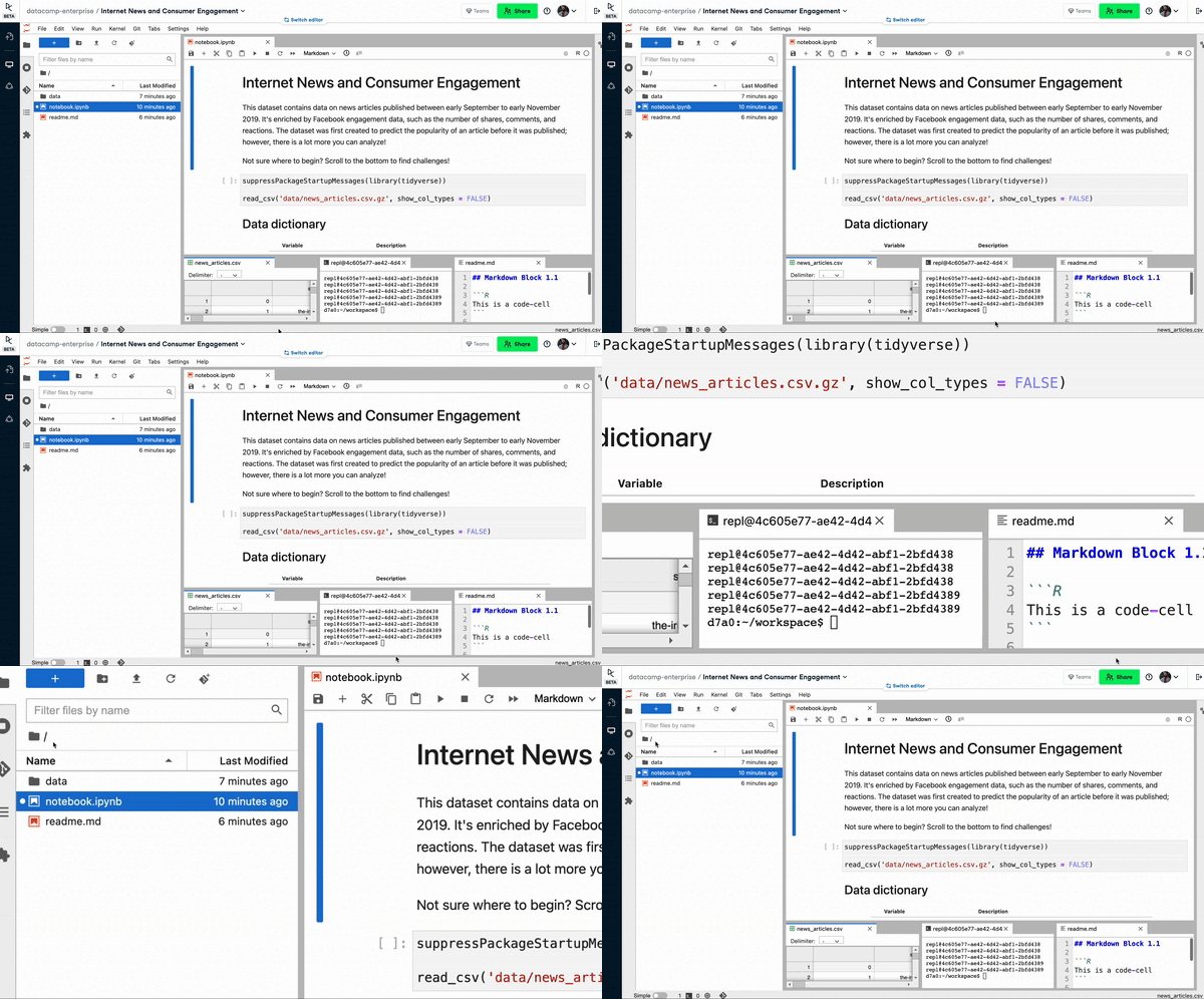
An overview of the JupyterLab interface on DataCamp Workspace
JupyterLab ≈ RStudio
Both JupyterLab and RStudio are popular Integrated Development Environments (IDE) for the R language. Save for some nuanced differences, they are very similar in function and feel. Among other things, RStudio comes with a file manager, terminal, a variable explorer, and even a function help pane. These allow programmers to access various files and settings easily, making analysis faster and easier. Many of these features can be found in JupyterLab too. In this section, we highlight the main components of the JupyterLab interface.
The Sidebar
The left sidebar contains five icons:
- A file browser, where you can open different files
- Running terminals and kernels, where you can see running processes
- Git, where you can manage repositories
- Table of content, where you can skim through notebook outlines
- Extension manager, where you can download notebook extensions
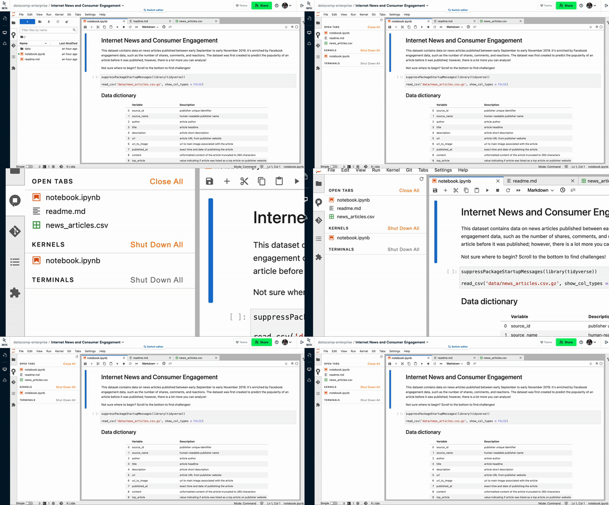 The file manager overview
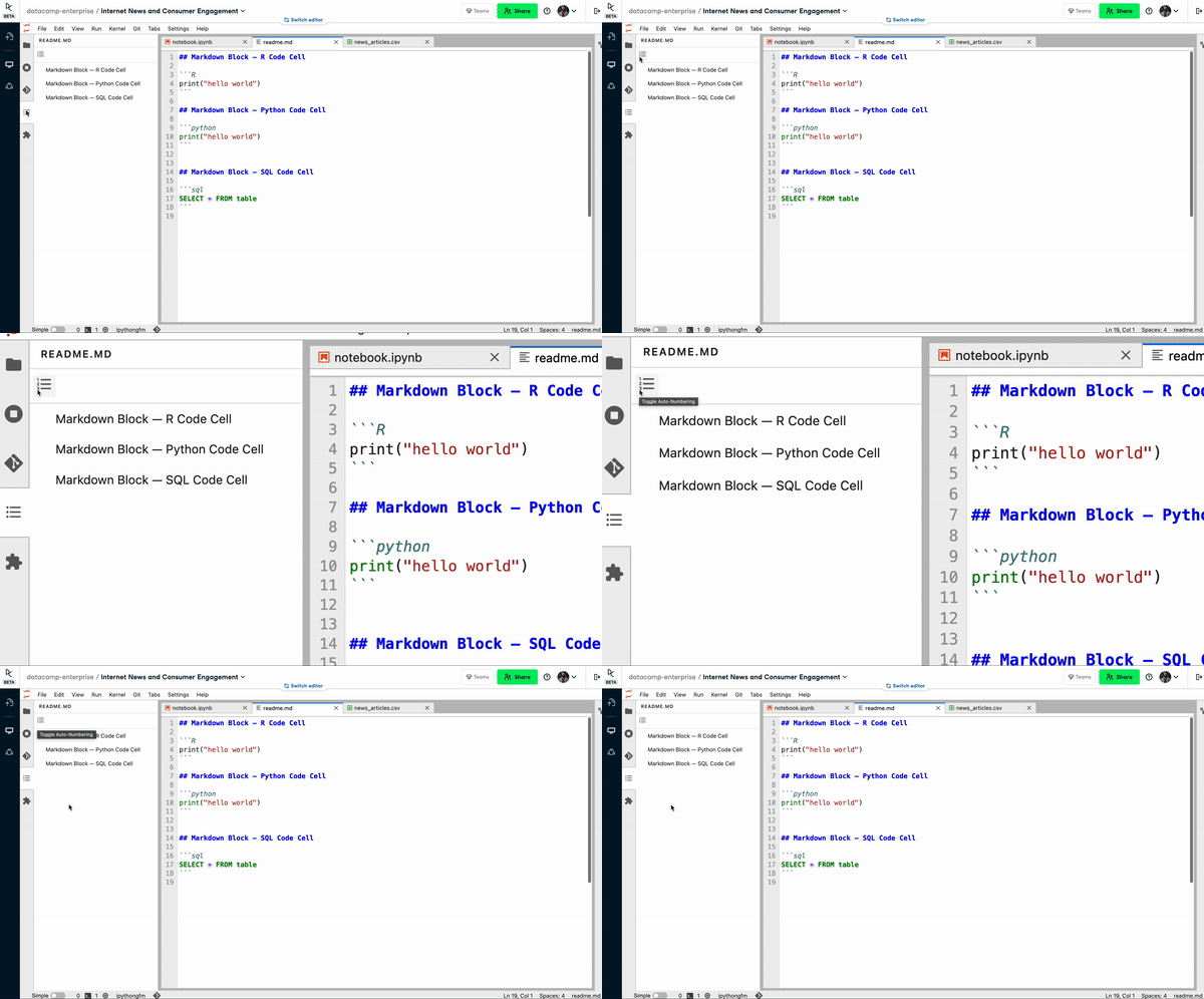 Running terminals and kernels

Table of contents overview
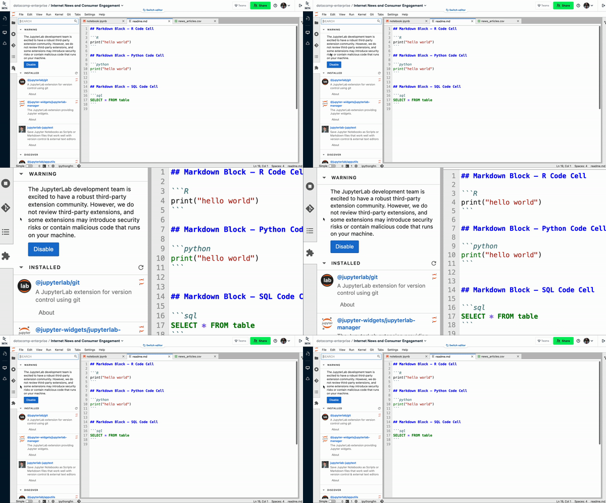
The extension manager overview
The Main Work Area
The main work area is where practitioners would write code, run shell commands, and edit markdown documentation. Much like RStudio, users can customize the layout to their liking. A practitioner can choose to focus on a single pane or work on several panes simultaneously.
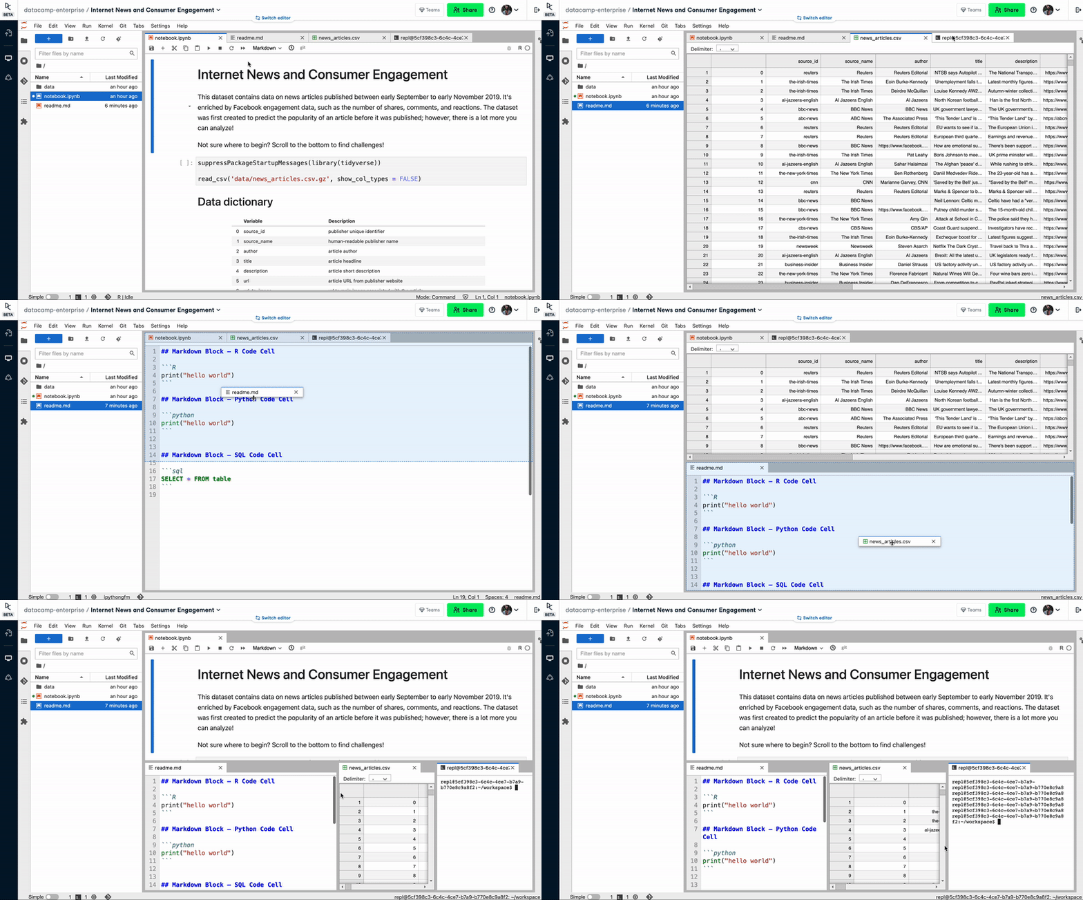
JupyterLab’s Customizable interface
Top Menu Bar
Just like RStudio, the top menu bar hosts a set of modals and ribbons that allow users to perform the following actions:
- File for opening, saving, and downloading notebooks amongst other actions
- Edit for editing cells content (like undo, redo, delete, and split cell)
- View for customizing the available panes in JupyterLab
- Run for running code blocks in Jupyter notebooks
- Kernel that interrupts or stops a kernel from running (we will discuss this later)
- Git for managing repositories and version control
- Tab allows users to navigate through the tabs in JupyterLab.
- Settings give users the flexibility of customizing the appearance of JupyterLab.
- Help contains more information on JupyterLab.
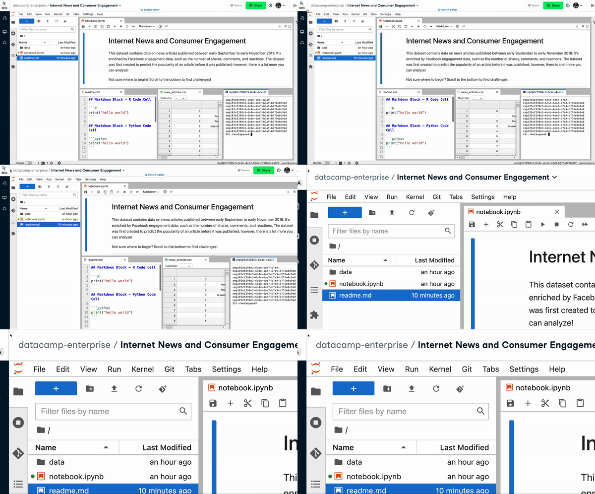
Top Menu Bar in JupyterLab
JupyterLab's Code Engine: The Kernel
A common term you may often read when working with Jupyter is “kernel”. A kernel is a process that executes code and interacts with Jupyter applications like JupyterLab. It can be thought of as the engine that runs the code contained in a Jupyter notebook. The kernel continues to run even when the notebook document, code console, or terminal is closed. This means that users can perform long-running actions (maybe close the notebook document) and return later.
To view all currently running Kernels, a user can navigate to the “Running Terminals and Kernels” tab. Here, the user can reopen the notebook linked to a given kernel.
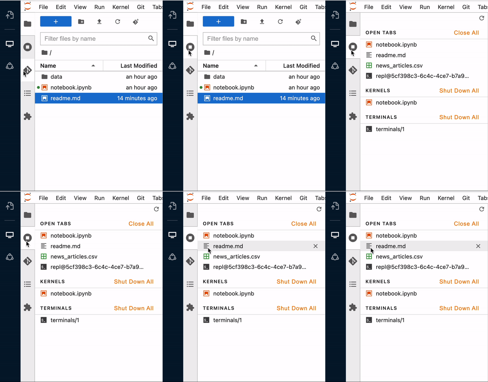
The running terminals and kernels side pane
There are a few kernel-related actions available to a user, including
- Interrupting a kernel: Doing so stops the code in the notebook from running, but keeps the variables of the notebook.
- Shut down a kernel: Doing so interrupts the kernel, and erases all the existing states and variables of the notebook.
- Restart a kernel: Doing so shuts down the existing kernel, and starts a new one.
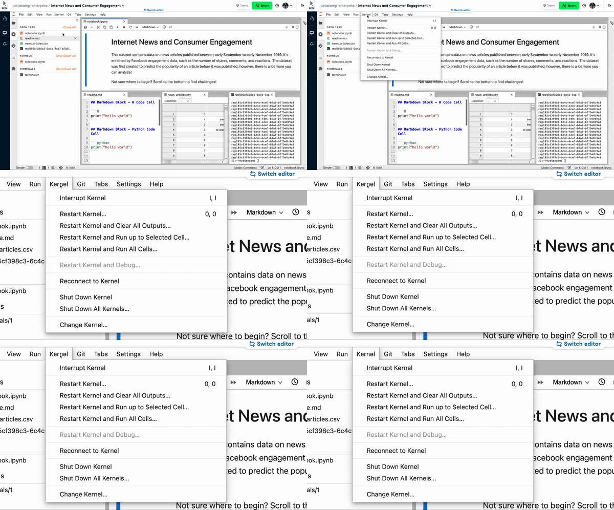
The kernel menu bar
Getting started with JupyterLab
Let’s walk through the process of creating a new notebook and running an analysis with JupyterLab. You can follow along with these instructions, by opening a new dataset or template using DataCamp Workspace.
Creating a Document
One can create a new notebook in JupyterLab using the menu File > New > Notebook. This is very much similar to RStudio. Alternatively, you can also press on the blue + on the top left-hand side to open new files.
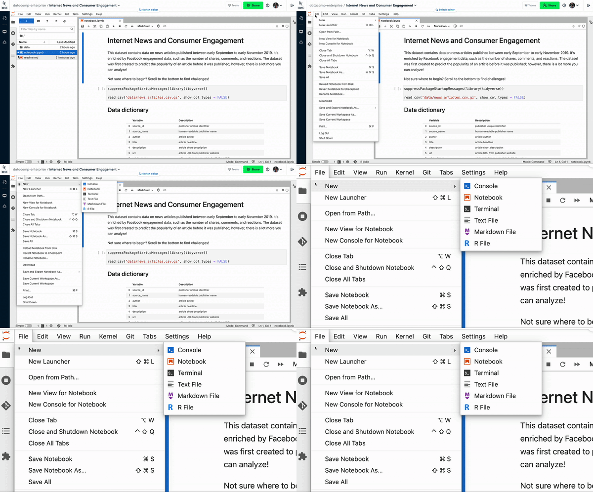
Opening a new file in JupyterLab
Writing and Running Code
A JupyterLab notebook consists of multiple blocks, each of which can contain either markdown or code. A code block in JupyterLab is similar to a chunk in RNotebook.
To create a block, one can click on the + button near the top of the console. You can run a code block by hitting the ▶ button (or Cmd+Enter for Macbook users, or Control+Enter for Windows users). Similar to RStudio, the output will be displayed underneath the code block upon running. Note that each code block is executed at once, like the ‘run current chunk’ function in RStudio.
In RStudio, each line can be run individually (Run > Run Selected Lines). Yet, the same can’t be said for JupyterLab. To run two lines individually, JupyterLab users must separate the lines into code blocks using the split cell function (Edit > Split Cell).
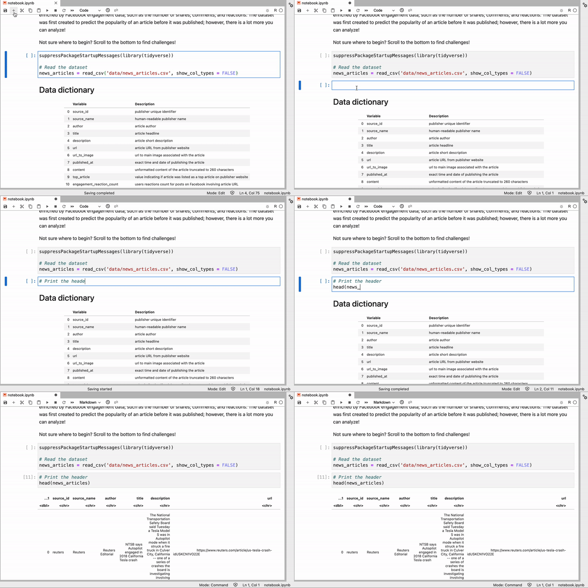
Running a code cell in JupyterLab
Managing Files
Similar to RStudio, JupyterLab has a file manager interface where users can navigate files and directories. Users can create, rename, move, and duplicate files.
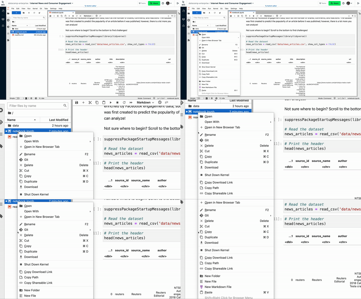
File manager in JupyterLab
Annotating code with Markdown
Annotations are a must-have in a readable notebook. In both Jupyter Notebook and RStudio, practitioners can provide context to their code with markdown segments.
To leverage markdown, JupyterLab users can create a new code block, and convert it to a Markdown block. Users can then use markdown syntax to decorate their text.
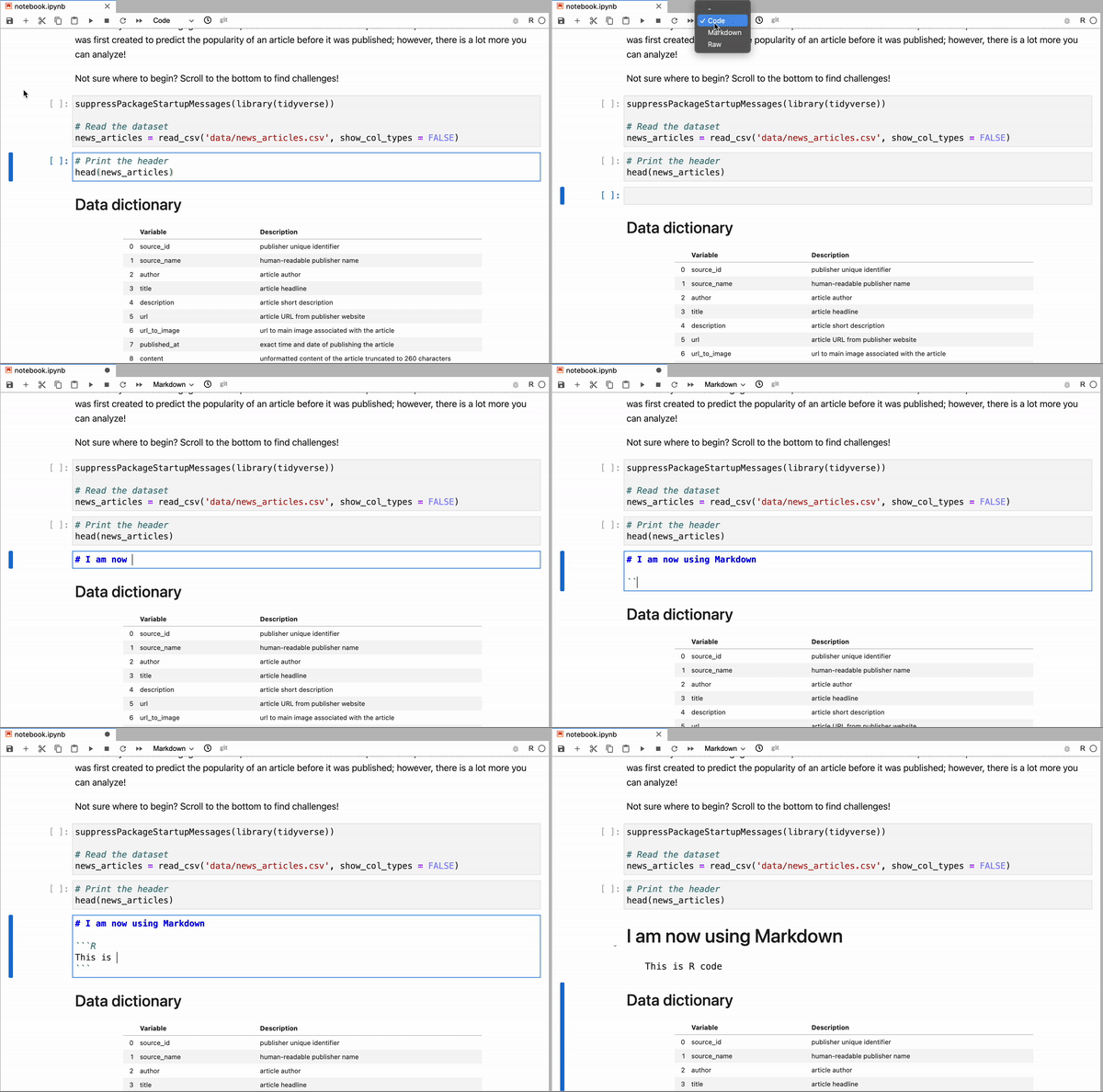
Using Markdown in JupyterLab
This is slightly different from RNotebook, where there is no need to create a separate block for markdown. Upon knitting, the notebook will be converted to an HTML document, where the code and markdown are displayed appropriately.
Saving and Publishing a Notebook
Saving in JupyterLab is similar to that in RStudio–both JupyterLab and RStudio automatically save the notebook at some default interval.
JupyterLab allows users to export Jupyter notebook files (.ipynb) to other formats, including HTML, LaTeX, Markdown, and PDF. To do so, simply go to File > Save and Export Notebook As… > Your ideal output format.
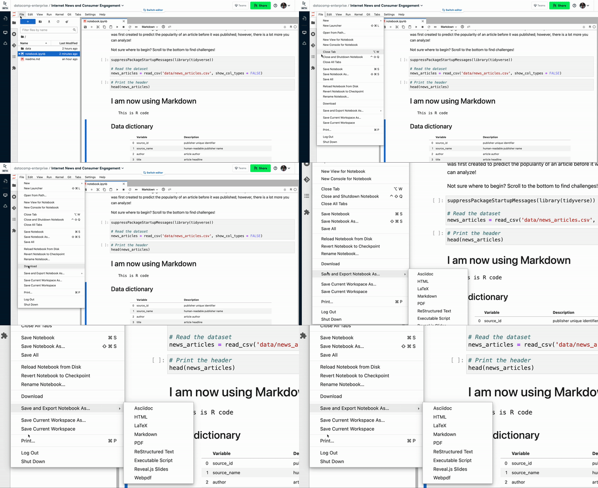
Saving and Exporting a Notebook
This is perhaps not a surprise for RStudio users. Upon previewing an RNotebook file, RStudio automatically saves an HTML webpage in the format of .nb.html.
Opening a Terminal and Code Console
The terminal is the interface for running shell commands. It comes in handy when a programmer needs to run R code and shell commands interactively. In JupyterLab, one can go to File > New > Terminal. This might be new to RStudio users, where the Terminal pane is on display by default.
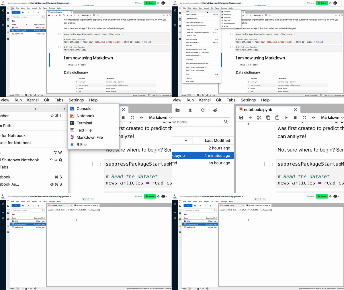 Opening a Terminal in JupyterLab
Customizing Themes
JupyterLab comes packaged with a default dark theme (Settings > Theme > Dark). Users can also install non-default themes using the Extension Manager.
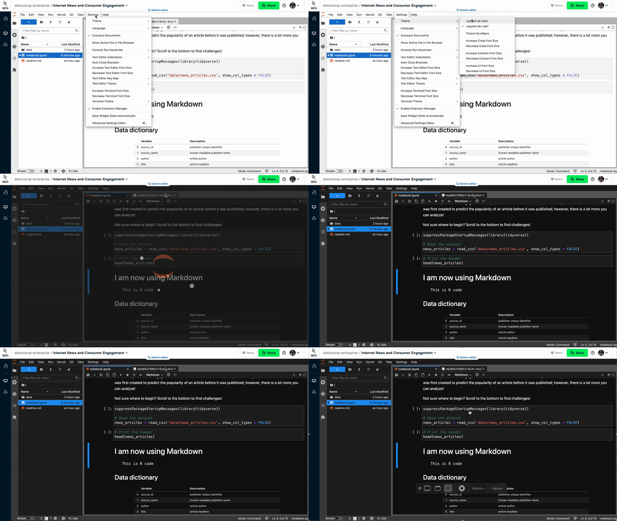
JupyterLab Dark Theme
JupyterLab vs RStudio
JupyterLab and RStudio are similar but not identical. Here we highlight two differences.
- Licenses: The Jupyter project is released under the modified BSD license. RStudio, on the other hand, is published under the Affero General Public Licenses.
- Features: Some Markdown features are not readily supported in Jupyter notebooks, including YAML headers for setting the theme, configuring the table of contents, advanced code appearance settings
Beyond JupyterLab and RStudio: The DataCamp Notebook Editor
While JupyterLab provides a host of useful features when working with data, we wanted to provide both Python and R data practitioners with additional benefits when working with DataCamp Workspace. This is why we released our very own DataCamp Notebook Editor.
The DataCamp Notebook Editor was built on top of Jupyter Notebooks, it allows teams to write code, analyze data, and share insights easily. It supports R, Python, and SQL. Here’s a run-down of key features of the DataCamp Notebook Editor.
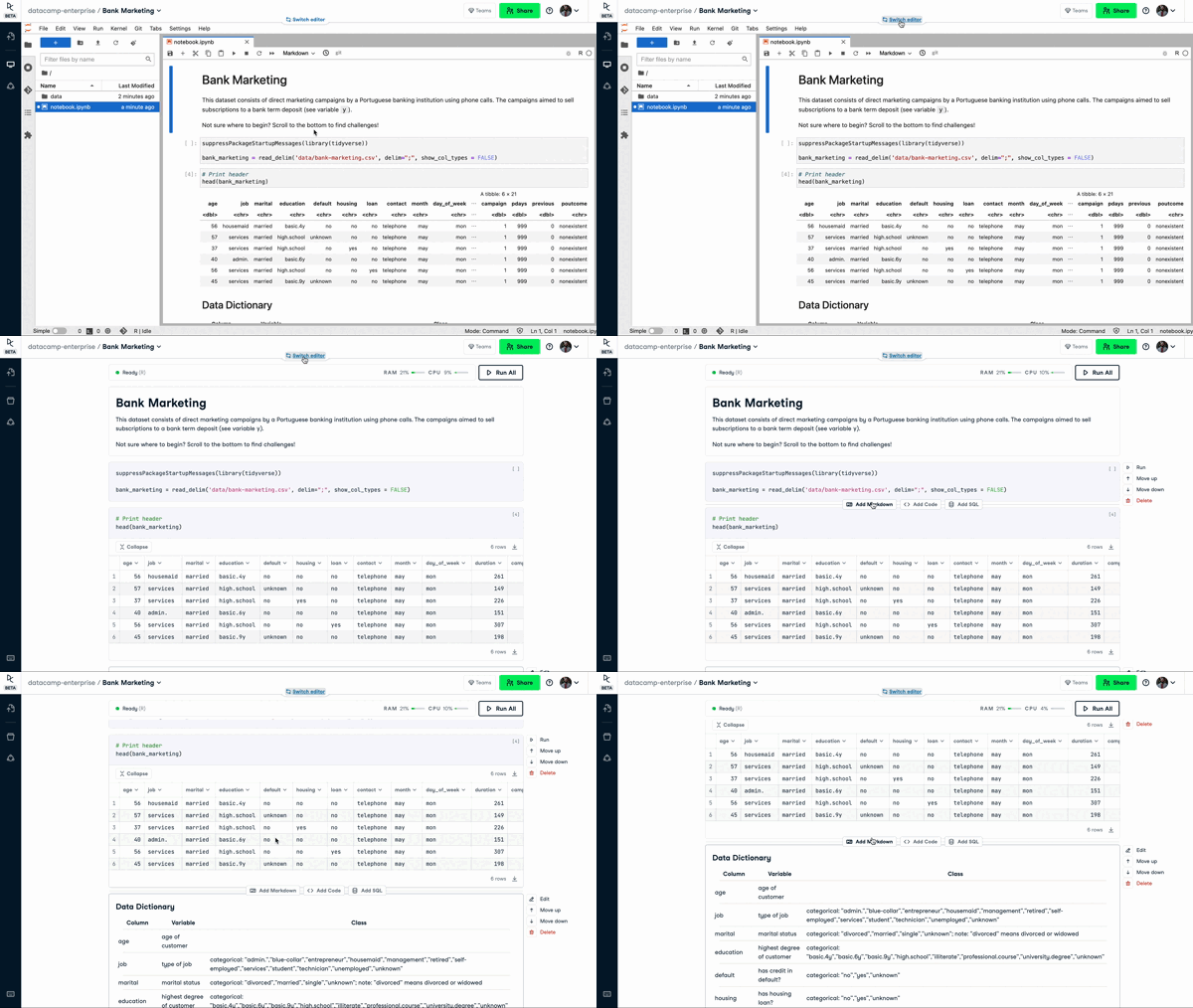
The DataCamp Notebook Editor
Easy Collaboration
Existing tools don’t always allow data scientists to edit the same code simultaneously. A bottleneck forms when data scientists start passing notebook files among one another. DataCamp Workspace addresses that head-on. It is a Google Docs for notebooks – multiple users can work on one notebook at any given time.
The notebook can be published and its link shared with a user’s teammates. Relaying a notebook that lives on the cloud is better than relaying an offline notebook, which might run on one local but not another.
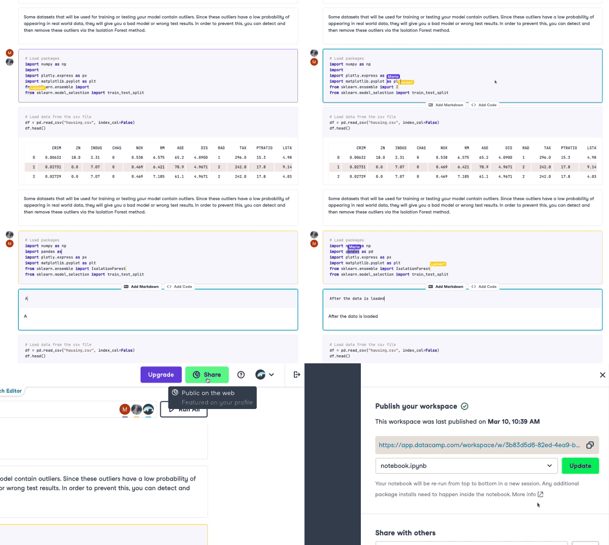
Collaboration in DataCamp Workspace
Native SQL Support
A handy feature in DataCamp Workspace is its native SQL support. Users can set up a secure connection from their DataCamp Notebook Editor to a database, like PostgreSQL, MySQL, and Redshift. Data extracted from the integrated database can then be analyzed using R or Python.
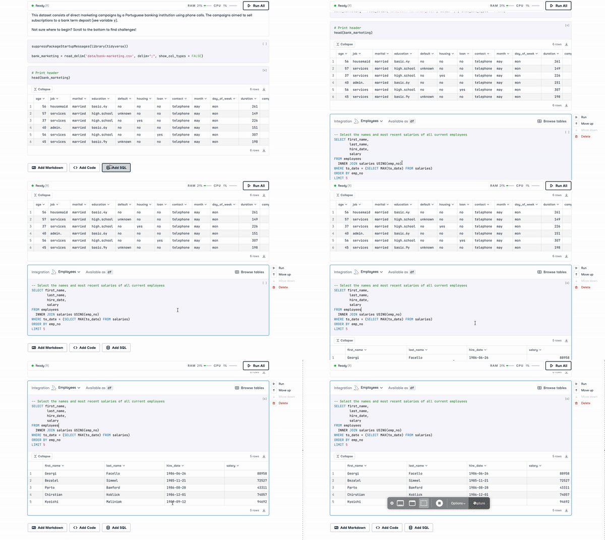
SQL in Workspace
Zero Setup
DataCamp Workspace and all of its features require no set-up. It’s on-demand, right at your fingertips, anytime. Whether using JupyterLab or the DataCamp Notebook Editor, you can open up Workspace on a web browser, and your notebook environment will go live in a matter of seconds. Since Workspace lives and runs on the cloud, you don’t need to download or install any additional software. In contrast, installing JupyterLab correctly on the browser is notoriously difficult, especially for beginner practitioners.
Get Started with DataCamp Workspace
We hope you enjoyed this run-down of how DataCamp Workspace can power your R Workflows. As we continue to improve existing features and build new features, make sure to let us know how we can create the best possible notebook environment for data practitioners.
Ready to go? Get coding with DataCamp Workspace now.

Filip is the passionate developer behind several of DataCamp's most popular Python, SQL, and R courses. Currently, Filip leads the development of DataLab, DataCamp's AI enabled data notebook. Filip holds degrees in Electrical Engineering and Artificial Intelligence.
