Decision Trees in Machine Learning Using R

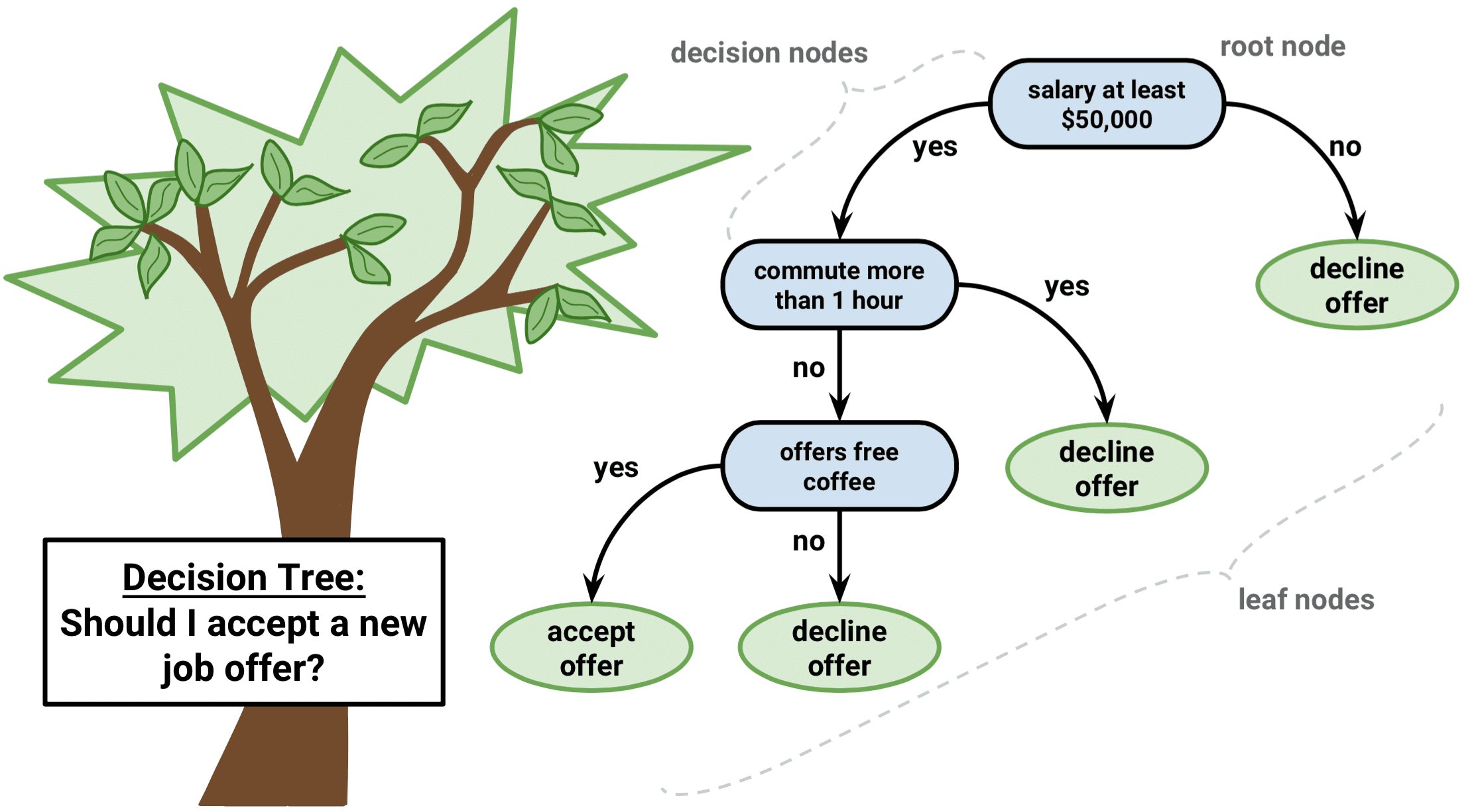
Picture yourself navigating through a maze. With every step, you face a decision that leads you closer to the exit or deeper into the labyrinth. This is akin to a decision tree algorithm, a powerful and intuitive machine learning method that helps us make sense of complex data and choose the best course of action.

A decision tree algorithm breaks down a dataset into smaller and smaller subsets based on certain conditions. Like a branching tree with leaves and nodes, it starts with a single root node and expands into multiple branches, each representing a decision based on a feature’s value. The final leaves of the tree are the possible outcomes or predictions.

This article will introduce you to the world of decision trees using the R programming language. We will discuss the basics, dive into popular types of decision tree algorithms, explore tree-based methods, and walk you through a step-by-step example. By the end, you’ll be able to harness the power of decision trees to make better data-driven decisions.

What is a Decision Tree in Machine Learning?

Decision trees are special in machine learning due to their simplicity, interpretability, and versatility.

It is a supervised machine learning algorithm that can be used for both regression (predicting continuous values) and classification (predicting categorical values) problems. Moreover, they serve as the foundation for more advanced techniques, such as bagging, boosting, and random forests.

This diagram below will illustrate the terminologies behind decision trees:

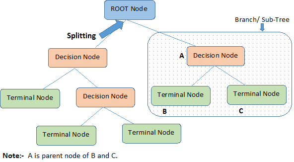
A decision tree starts with a root node that signifies the whole population or sample, which then separates into two or more uniform groups via a method called splitting. When sub-nodes undergo further division, they are identified as decision nodes, while the ones that don't divide are called terminal nodes or leaves. A segment of a complete tree is referred to as a branch.

We established that decision trees could be used for both regression and classification tasks; thus, let’s understand the algorithm behind the types of decision trees.

Popular Types of Decision Trees Algorithms

Let’s intuitively understand both regression and classification decision trees, what’s similar and different in each, and the error functions.

Regression Trees

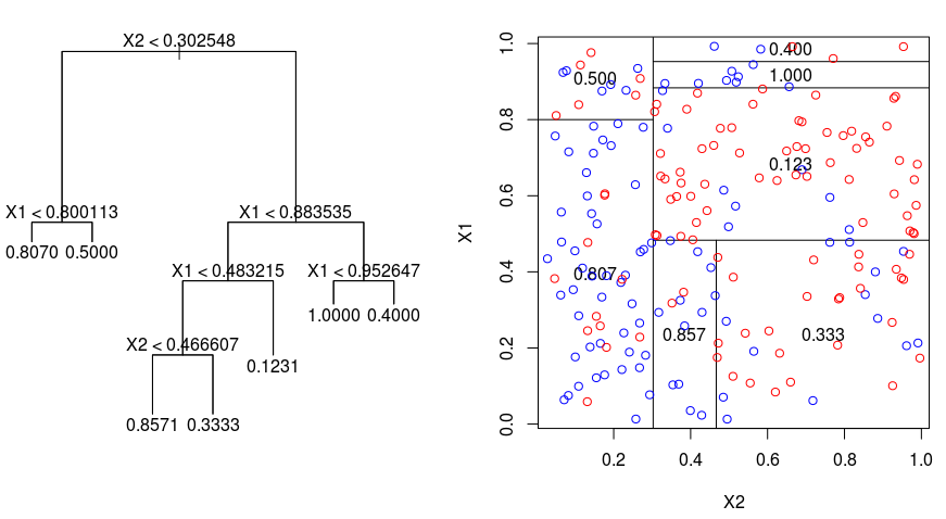
Let's take a look at the image below, which helps visualize the nature of partitioning carried out by a Regression Tree. This shows an unpruned tree and a regression tree fit to a random dataset. Both the visualizations show a series of splitting rules, starting at the top of the tree. Notice that every split of the domain is aligned with one of the feature axes. The concept of axis parallel splitting generalizes straightforwardly to dimensions greater than two. For a feature space of size $p$, a subset of $\mathbb{R}^p$, the space is divided into $M$ regions, $R_{m}$, each of which is a $p$-dimensional "hyperblock".

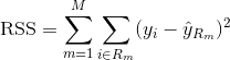
In order to build a regression tree, you first use recursive binary splitting to grow a large tree on the training data, stopping only when each terminal node has fewer than some minimum number of observations. Recursive Binary Splitting is a greedy and top-down algorithm used to minimize the Residual Sum of Squares (RSS), an error measure also used in linear regression settings. The RSS, in the case of a partitioned feature space with M partitions is given by:

Beginning at the top of the tree, you split it into 2 branches, creating a partition of 2 spaces. You then carry out this particular split at the top of the tree multiple times and choose the split of the features that minimizes the (current) RSS.

Next, you apply cost complexity pruning to the large tree in order to obtain a sequence of best subtrees, as a function of $\alpha$. The basic idea here is to introduce an additional tuning parameter, denoted by $\alpha$ that balances the depth of the tree and its goodness of fit to the training data.

You can use K-fold cross-validation to choose $\alpha$. This technique simply involves dividing the training observations into K folds to estimate the test error rate of the subtrees. Your goal is to select the one that leads to the lowest error rate.

Classification Trees

A classification tree is very similar to a regression tree, except that it is used to predict a qualitative response rather than a quantitative one.

Recall that for a regression tree, the predicted response for an observation is given by the mean response of the training observations that belong to the same terminal node. In contrast, for a classification tree, you predict that each observation belongs to the most commonly occurring class of training observations in the region to which it belongs.

In interpreting the results of a classification tree, you are often interested not only in the class prediction corresponding to a particular terminal node region, but also in the class proportions among the training observations that fall into that region.

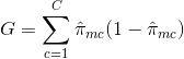
The task of growing a classification tree is quite similar to the task of growing a regression tree. Just as in the regression setting, you use recursive binary splitting to grow a classification tree. However, in the classification setting, the Residual Sum of Squares cannot be used as a criterion for making the binary splits. Instead, you can use either of these 3 methods below:

• Classification Error Rate: Rather than seeing how far a numerical response is away from the mean value, as in the regression setting, you can instead define the "hit rate" as the fraction of training observations in a particular region that doesn't belong to the most widely occurring class. The error is given by this equation:

E = 1 - argmax_c($\hat{\pi}_{mc}$)

in which $\hat{\pi}_{mc}$ represents the fraction of training data in region R_m that belong to class c.

• Gini Index: The Gini Index is an alternative error metric that is designed to show how "pure" a region is. "Purity" in this case means how much of the training data in a particular region belongs to a single class. If a region R_m contains data that is mostly from a single class c then the Gini Index value will be small:

• Cross-Entropy: A third alternative, which is similar to the Gini Index, is known as the Cross-Entropy or Deviance:

The cross-entropy will take on a value near zero if the $\hat{\pi}_{mc}$’s are all near 0 or near 1. Therefore, like the Gini index, the cross-entropy will take on a small value if the mth node is pure. In fact, it turns out that the Gini index and the cross-entropy are quite similar numerically.

When building a classification tree, either the Gini index or the cross-entropy are typically used to evaluate the quality of a particular split, since they are more sensitive to node purity than is the classification error rate. Any of these 3 approaches might be used when pruning the tree, but the classification error rate is preferable if prediction accuracy of the final pruned tree is the goal.

Advantages and Disadvantages of Decision Trees

As much as we’d like to understand the algorithm and its strengths, it's crucial to understand its shortcomings. The truth is that decision trees aren’t the best fit for all types of machine learning algorithms, which is also the case for all machine learning algorithms.

Here are the advantages and disadvantages:

Advantages

1. Easy to understand and interpret. Decision trees are highly intuitive and can be easily visualized. Their hierarchical structure resembles human decision-making, making them accessible even to non-experts. This interpretability is crucial in situations where understanding the decision process is just as important as the prediction itself.
2. Can handle both continuous and categorical variables. Decision trees are versatile and can manage datasets with a mix of continuous and categorical features, as well as target variables of either type. This flexibility allows decision trees to be applied to a wide range of problems.
3. Minimal data preprocessing is required. Decision trees do not require feature scaling or normalization, as they are invariant to monotonic transformations. They can also easily handle missing values and outliers, making them suitable for raw and noisy data.
4. Can be used for feature selection and identifying important variables. Decision trees naturally perform feature selection by choosing the most informative features for splitting the data. The importance of a feature can be determined based on how early it appears in the tree and how often it is used for splitting.

Disadvantages

1. Prone to overfitting. Decision trees can become overly complex when they grow deep, leading to overfitting the training data. This results in poor generalization of unseen data. Techniques such as pruning or setting a maximum depth can help mitigate this issue.
2. Sensitive to small changes in the data. A small change in the training data can lead to a completely different tree structure, making decision trees unstable. This sensitivity can be reduced by ensemble methods, such as bagging, boosting, or random forests, which build multiple trees and aggregate their results.
3. Decision tree models are often not as accurate as other machine learning methods. Due to their simplicity and the greedy nature of their construction, decision trees may not always produce the most accurate models. However, they can serve as a good starting point or baseline model for comparison with more sophisticated methods.
4. Biased towards dominant classes. Decision trees can be biased towards the majority class in imbalanced datasets, leading to suboptimal splits and misclassification of minority instances. Techniques such as oversampling, undersampling, or using cost-sensitive learning can help address this issue.

Despite these disadvantages, decision trees remain a popular choice in many applications due to their simplicity, interpretability, and versatility.

Advanced Tree-Based Machine Learning Algorithms

Let’s explore tree-based ensemble methods that leverage the strengths of decision trees while addressing some of their limitations: bagging, boosting, and random forests.

Bagging

The decision trees discussed above suffer from high variance, meaning if you split the training data into 2 parts at random, and fit a decision tree to both halves, the results that you get could be quite different. In contrast, a procedure with low variance will yield similar results if applied repeatedly to distinct dataset.

Bagging, or bootstrap aggregation, is a technique used to reduce the variance of your predictions by combining the result of multiple classifiers modeled on different sub-samples of the same dataset. Here is the equation for bagging:

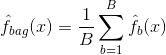
in which you generate $B$ different bootstrapped training datasets. You then train your method on the $bth$ bootstrapped training set in order to get $\hat{f}_{b}(x)$, and finally average the predictions.

The visual below shows the 3 different steps in bagging:

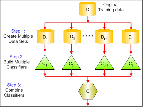
• Step 1: Here you replace the original data with new data. The new data usually have a fraction of the original data's columns and rows, which then can be used as hyper-parameters in the bagging model.

• Step 2: You build classifiers on each dataset. Generally, you can use the same classifier for making models and predictions.

• Step 3: Lastly, you use an average value to combine the predictions of all the classifiers, depending on the problem. Generally, these combined values are more robust than a single model.

While bagging can improve predictions for many regression and classification methods, it is particularly useful for decision trees. To apply bagging to regression/classification trees, you simply construct $B$ regression/classification trees using $B$ bootstrapped training sets, and average the resulting predictions. These trees are grown deep, and are not pruned. Hence each individual tree has high variance, but low bias. Averaging these $B$ trees reduces the variance.

Broadly speaking, bagging has been demonstrated to give impressive improvements in accuracy by combining together hundreds or even thousands of trees into a single procedure.

Random Forests

Random Forests is a versatile machine learning method capable of performing both regression and classification tasks. It also undertakes dimensional reduction methods, treats missing values, outlier values, and other essential steps of data exploration, and does a fairly good job.

Random Forests improves bagged trees by a small tweak that decorrelates the trees. As in bagging, you build a number of decision trees on bootstrapped training samples. But when building these decision trees, each time a split in a tree is considered, a random sample of m predictors is chosen as split candidates from the full set of $p$ predictors. The split is allowed to use only one of those $m$ predictors. This is the main difference between random forests and bagging; because as in bagging, the choice of predictor $m = p$.

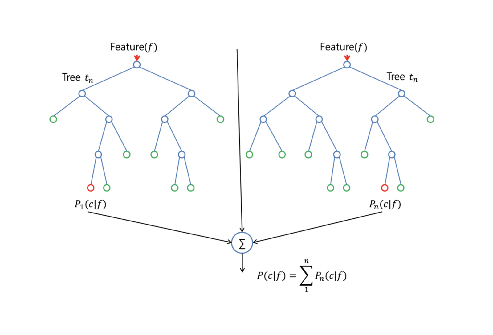
In order to grow a random forest, you should:

• First assume that the number of cases in the training set is K. Then, take a random sample of these K cases, and then use this sample as the training set for growing the tree.

• If there are $p$ input variables, specify a number $m < p$ such that at each node, you can select $m$ random variables out of the $p$. The best split on these $m$ is used to split the node.

• Each tree is subsequently grown to the largest extent possible and no pruning is needed.

• Finally, aggregate the predictions of the target trees to predict new data.

Random Forests is very effective at estimating missing data and maintaining accuracy when a large proportions of the data is missing. It can also balance errors in datasets where the classes are imbalanced. Most importantly, it can handle massive datasets with large dimensionality. However, one disadvantage of using Random Forests is that you might easily overfit noisy datasets, especially in the case of doing regression.

Boosting

Boosting is another approach to improve the predictions resulting from a decision tree. Like bagging and random forests, it is a general approach that can be applied to many statistical learning methods for regression or classification. Recall that bagging involves creating multiple copies of the original training dataset using the bootstrap, fitting a separate decision tree to each copy, and then combining all of the trees in order to create a single predictive model. Notably, each tree is built on a bootstrapped dataset, independent of the other trees.

Boosting works in a similar way, except that the trees are grown sequentially: each tree is grown using information from previously grown trees. Boosting does not involve bootstrap sampling; instead, each tree is fitted on a modified version of the original dataset.

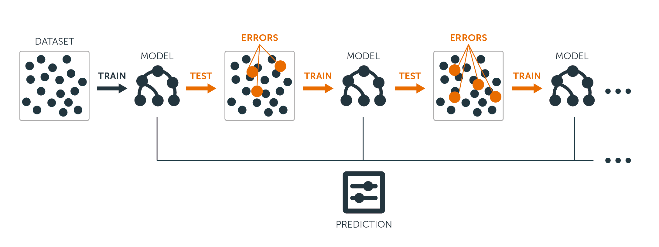
For both regression and classification trees, boosting works like this:

• Unlike fitting a single large decision tree to the data, which amounts to fitting the data hard and potentially overfitting, the boosting approach instead learns slowly.

• Given the current model, you fit a decision tree to the residuals from the model. That is, you fit a tree using the current residuals, rather than the outcome $Y$, as the response.

• You then add this new decision tree into the fitted function in order to update the residuals. Each of these trees can be rather small, with just a few terminal nodes, determined by the parameter $d$ in the algorithm. By fitting small trees to the residuals, you slowly improve $\hat{f}$ in areas where it does not perform well.

• The shrinkage parameter $\nu$ slows the process down even further, allowing more and different shaped trees to attack the residuals.

Boosting is very useful when you have a lot of data and you expect the decision trees to be very complex. Boosting has been used to solve many challenging classification and regression problems, including risk analysis, sentiment analysis, predictive advertising, price modeling, sales estimation, and patient diagnosis, among others.

Essentially these algorithms combine the predictions of multiple decision trees to improve overall performance and stability. Having understood the advanced algorithms, for the scope of this tutorial, we’ll proceed with the simple decision tree models.

Building Decision Tree Models Step-by-Step in R

We’ve learned plenty of theory and the intuition behind decision tree models and their variations, but nothing beats going hands-on and building those models, evaluating their model performance in a step-by-step fashion.

Preparing the data for modeling

For the following examples, we’ll use the popular Boston Housing Dataset.

The Boston Housing dataset contains information about the housing market in Boston, Massachusetts, in the 1970s. It has 506 observations and 14 variables, including 13 features and 1 target variable.

The features in the Boston Housing dataset are:

• CRIM: Per capita crime rate by town
• ZN: Proportion of residential land zoned for lots over 25,000 sq.ft.
• INDUS: Proportion of non-retail business acres per town
• CHAS: Charles River dummy variable (= 1 if tract bounds river; 0 otherwise)
• NOX: Nitric oxide concentration (parts per 10 million)
• RM: Average number of rooms per dwelling
• AGE: Proportion of owner-occupied units built before 1940
• DIS: Weighted distances to five Boston employment centers
• RAD: Index of accessibility to radial highways
• TAX: Full-value property tax rate per $10,000
• PTRATIO: Pupil-teacher ratio by town
• Black: proportion of Black people by town
• LSTAT: Percentage of the lower status of the population

The target variable is MEDV which represents the Median value of owner-occupied homes in $1000s.

The goal is to predict the median value of owner-occupied homes (in thousands of dollars) based on the given features.

In R, the data is provided in a package called “MASS.” You will have to install multiple packages for this tutorial and load them. Since this would be a repetition, let’s demonstrate this process with the MASS package once, and you’ll repeat it whenever you see a new package used in this guide.

# install the package
install.packages("MASS")

# Load the MASS package
library(MASS)

# Load the Boston Housing dataset
data(Boston)

It’s often necessary to explore the data through visualizations and perform data pre-processing steps before moving into modeling. Let’s have a look at the distribution of the variables through histograms.

Here’s the code to create them:

# Load the library
library(tidymodels)
library(tidyr)

# Prepare the dataset for ggplot2
boston_data_long <- Boston %>%
 pivot_longer(cols = everything(),
              names_to = "variable",
              values_to = "value")

# Create a histogram for all numeric variables in one plot
boston_histograms <- ggplot(boston_data_long, aes(x = value)) +
 geom_histogram(bins = 30, color = "black", fill = "lightblue") +
 facet_wrap(~variable, scales = "free", ncol = 4) +
 labs(title = "Histograms of Numeric Variables in the Boston Housing Dataset",
      x = "Value",
      y = "Frequency") +
 theme_minimal()

# Plot the histograms
print(boston_histograms)

And the output looks like this:

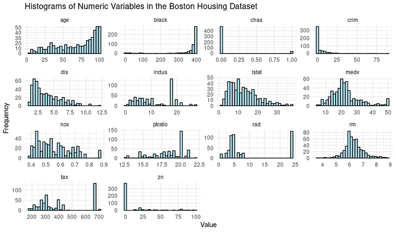
We do notice some outliers, especially in the columns such as RAD, TAX and NOX. Our goal for this tutorial is to focus on the decision tree modeling phase; hence let’s split the dataset into training and testing sets.

# Split the data into training and testing sets

set.seed(123)
data_split <- initial_split(Boston, prop = 0.75)
train_data <- training(data_split)
test_data <- testing(data_split)

Let’s now dive into modeling and evaluating the model performance.

Simple Decision Tree Modelling

Using the function decision_tree() from the Tidymodels package in R, it is straightforward to create a decision tree model specification first and then fit the model on the training data.

# Create a decision tree model specification
tree_spec <- decision_tree() %>%
 set_engine("rpart") %>%
 set_mode("regression")

# Fit the model to the training data
tree_fit <- tree_spec %>%
 fit(medv ~ ., data = train_data)

We use the “regression” model here, and for a classification decision tree, we would have to use the “classification” mode.

Evaluating the Decision Treel Modelling Performance

To evaluate the model’s performance, we will use the Tidymodels package to calculate the root mean squared error (RMSE) and the R-squared value for our decision tree model on the testing data.

# Make predictions on the testing data
predictions <- tree_fit %>%
 predict(test_data) %>%
 pull(.pred)

# Calculate RMSE and R-squared
metrics <- metric_set(rmse, rsq)
model_performance <- test_data %>%
 mutate(predictions = predictions) %>%
 metrics(truth = medv, estimate = predictions)

print(model_performance)

You’d get an output presenting two performance metrics: Root Mean Squared Error (RMSE) and R-squared (R²).

 .metric .estimator .estimate
 <chr>   <chr>          <dbl>
1 rmse    standard       5.22
2 rsq     standard       0.689

Analyzing the Model Results

So, are our model results good enough?

• RMSE (Root Mean Squared Error): This measures the average difference between the predicted and true values. In your case, the RMSE is 5.22, which means that, on average, the predictions made by the decision tree model are off by approximately 5.22 units from the true values. A lower RMSE value is generally better, as it indicates smaller prediction errors.
• R-squared (R²): This measures how well the model explains the variance in the target variable. It ranges from 0 to 1, with a higher value indicating a better fit. In your case, the R² is 0.689, meaning the model explains approximately 68.9% of the variance in the target variable (MEDV).

We can also optimize the hyper-parameters to squeeze out performance or go for more complex models such as Random Forests and XGBoost at the cost of model interpretability.

Predicting Outcomes Using the Decision Tree Model

Once you’re happy with the model, it’s time to let the model make predictions.

This is the same as how we did with the test data using the predict() function, but we’ll have to provide a new set of data mimicking information about a new house in Boston. It’s a possible scenario when the model goes live in a production environment.

# Make predictions on new data
new_data <- tribble(
 ~crim, ~zn, ~indus, ~chas, ~nox, ~rm, ~age, ~dis, ~rad, ~tax, ~ptratio, ~black, ~lstat,
 0.03237, 0, 2.18, 0, 0.458, 6.998, 45.8, 6.0622, 3, 222, 18.7, 394.63, 2.94
)
predictions <- predict(tree_fit, new_data)
print(predictions)

And you’ll get the predicted medium value (in $1000s) of this particular house:

# A tibble: 1 × 1
 .pred
 <dbl>
1  37.8

With that, you’re equipped with the steps of building a decision tree model — let’s now focus on how we can interpret what’s going inside the model for ourselves and the stakeholder who use the solution we just built.

Interpreting the Decision Tree

The most significant advantage, as we stated earlier, is the interpretability of the decision tree models. Let’s visualize the decision tree to understand the model better:

# Load the library
library(rpart.plot)

# Plot the decision tree
rpart.plot(tree_fit$fit, type = 4, extra = 101, under = TRUE, cex = 0.8, box.palette = "auto")

You will see a plot like this:

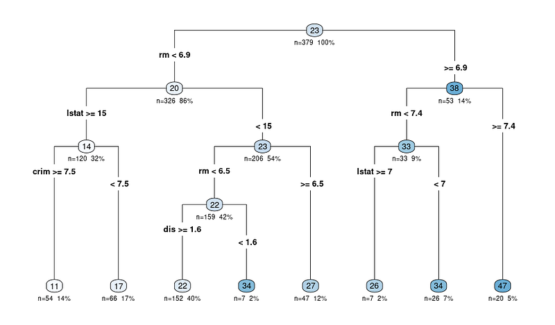
The output diagram of the rpart.plot function shows a decision tree representation of the model. In this diagram, each node represents a split in the decision tree based on the predictor variables. The output diagram includes several pieces of information that can help us interpret the decision tree:

The tree diagrams start with the node

The nodes are represented by circles and are connected by lines, showing the hierarchical structure of the decision tree. The tree starts with a root node at the top, and it branches into internal nodes, ultimately leading to the terminal nodes or leaves at the bottom.

The splitting criteria for each internal node

Each internal node displays the splitting criterion, which is the predictor variable and the value used to split the data into two subsets.

For example, a node might show “RM < 6.8”, indicating that observations with an average number of rooms per dwelling (RM) less than 6.8 will follow the left branch, while observations with RM greater than or equal to 6.8 will follow the right branch.

N: Number of observations after the split

The n value in each node represents the number of observations in the dataset that fall into that particular node. For example, if a node shows "n = 100", it means that 100 observations in the dataset meet the criteria of that node's parent nodes.

X%: The proportion of the total dataset observations that reached the particular node.

The percentage value helps you understand the relative size of each node compared to the entire dataset, showing how the data is being split and distributed across the tree. A higher percentage means a larger proportion of the data has followed the decision path leading to the specific node, while a lower percentage indicates a smaller proportion of the data reaching that node.

The predicted value for each node

The predicted value at each node is displayed as a number in a colored circle (node). In a regression tree, this is the average target variable value for all observations that fall into that node.

For example, the last lead node showing 47 means that the average target variable value (in our case, the median value of owner-occupied homes) for all observations in that node is 47.

Start at the root node and follow the branches

So when interpreting any outcomes, you start at the root node and follow the branches based on the splitting criteria until you reach a terminal node. The predicted value in the terminal node gives the model’s prediction for a given observation and the rationale behind the decision.

Extracting the rules from the decision tree

If you still prefer to extract the rules in text form (instead of traversing through the diagram) — you can do this, too, using the same library we used to plot the diagram.

Here’s the code to do it:

rules <- rpart.rules(tree_fit$fit)
print(rules)

And you’ll see an output with the predicted values and rules it follows to arrive at that value as below:

medv                                                              
  11 when rm <  6.9        & lstat >= 15 & crim >= 7.5            
  17 when rm <  6.9        & lstat >= 15 & crim <  7.5            
  22 when rm <  6.5        & lstat <  15               & dis >= 1.6
  26 when rm is 6.9 to 7.4 & lstat >=  7                          
  27 when rm is 6.5 to 6.9 & lstat <  15                          
  34 when rm <  6.5        & lstat <  15               & dis <  1.6
  34 when rm is 6.9 to 7.4 & lstat <   7                          
  47 when rm >=        7.4

Now that you see the rules, you might wonder how the decision can be made with 3–4 variables when we feed many more variables to the decision tree.

Well, turns out some variables are more important than the rest. Let’s understand this concept better.

Understanding the Important Variables from Decision Trees

We’ve already uncovered the tree diagram and how the model works. One last aspect of the interpretation is understanding the important variables from the dataset.

Here’s why it’s crucial:

• Feature selection. Identifying important variables can help you focus on relevant features and potentially remove less important ones, simplifying your model and reducing noise.
• Domain knowledge. Gaining insights into which features are most important can help you better understand the relationships between variables and the target variable in the context of your specific problem.
• Model interpretation. Understanding the key features driving the model’s predictions can provide valuable insights into the decision-making process.

In decision trees, variable importance is usually determined by the features used for splitting at the nodes. Features that are used for splitting higher up in the tree or used more frequently can be considered more important.

The importance of a variable can be quantified by the reduction in the impurity measure (e.g., Gini index or mean squared error) it brings when used for splitting. The “VIP” package in R has taken out all the complexities, and the plot can be obtained through the code below:

# Load the necessary library
library(vip)

# Create a variable importance plot
var_importance <- vip::vip(tree_fit, num_features = 10)
print(var_importance)

And you’ll get the variable importance plot below:

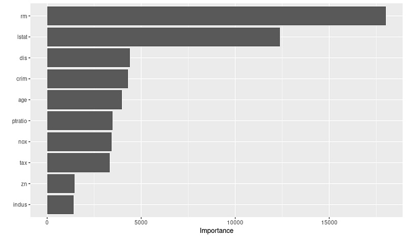
Once you see the plot, you could do further research as to why these variables are important, collaborating with domain experts. For example, based on the above plot, we can infer the top 3 important variables and the rationale:

1. RM: The average number of rooms per dwelling is a highly crucial feature, suggesting that houses with more rooms tend to have higher median values.
2. LSTAT: The percentage of the population with lower socioeconomic status is another significant variable, indicating that lower-status neighborhoods are likely to have lower median home values.
3. DIS: The weighted distance to employment centers is a vital variable, showing that houses closer to major employment centers are likely to have higher median values.

So remember to check the variable importance plot before finalizing your model; this can help you create and select better features to optimize the performance.

Conclusion

In this tutorial, we have explored the fundamental concepts of decision trees and approached not just building models but also interpreting them. Decision trees are powerful and interpretable models for both classification and regression tasks, making them an essential tool in a data scientist’s arsenal.

As you continue to develop your skills, we encourage you to dive deeper into the world of decision trees, explore alternative algorithms, and enhance your R programming abilities. Here are some resources for your next step:

• Machine Learning Fundamentals in R
• Introduction to Feature Engineering in R
• Modelling with Tidymodels in R
• Machine Learning with Tree-based Models in R

Without any doubt, expanding your knowledge and experimenting with new tools and techniques will enable you to tackle diverse challenges and provide valuable insights into your projects.