Markov Chain Analysis in R

What is a Markov Chain?

A Markov Chain is a mathematical system that experiences transitions from one state to another according to a given set of probabilistic rules. Markov chains are stochastic processes, but they differ in that they must lack any "memory". That is, the probability of the next state of the system is only dependent on the present state of the system and not on any prior states. This is called the Markov property (seen below):

In order to have a functional Markov chain model, it is essential to define a transition matrix P_^t. A transition matrix contains the information about the probability of transitioning between the different states in the system. For a transition matrix to be valid, each row must be a probability vector, and the sum of all its terms must be 1.

Transition Matrices have the property that the product of subsequent matrices can describe the transition probabilities along a time interval. Therefore, one can model how probable is to be at a certain state after k steps by calculating the following:

This tutorial will also cover absorbing Markov chains. These chains occur when there is at least one state that, once reached, the probability of staying on it is 1 (you cannot leave it).

What are Absorbing Markov Chains?

An absorbing Markov chain is a Markov chain in which it is impossible to leave some states once entered. However, this is only one of the prerequisites for a Markov chain to be an absorbing Markov chain. In order for it to be an absorbing Markov chain, all other transient states must be able to reach the absorbing state with a probability of 1.

Absorbing Markov chains have specific unique properties that differentiate them from the normal time-homogeneous Markov chains. One of these properties is the way in which the transition matrix can be written. With a chain with t transient states and r absorbing states, the transition matrix P can be written in canonical form as follows:

Where Q is a t x t matrix, R is a t x r matrix, 0 is a r x t zero matrix, and I_^r is a r x r identity matrix. In particular, the decomposition of the transition matrix into the fundamental matrix allows for certain calculations such as the expected number of steps until absorption from each state. The fundamental matrix N is calculated as follows:

Where I_^t is a t x t identity matrix

The expected number of steps is based on the concept of linearity of expectation, and it is calculated as follows:

Where 1 is a column vector of the same length as the number of transient states with all entries being 1

Furthermore, we can calculate the probability of being absorbed by a specific absorbing state when starting from any given transient state. This probability is calculated as follows:

Analysis of Sales Velocity

Markov chains are widely used in many fields such as finance, game theory, and genetics. However, the basis of this tutorial is how to use them to model the length of a company's sales process since this could be a Markov process. This was in fact validated by testing if sequences are detailing the steps that a deal went through before successfully closing complied with the Markov property.

This analysis carried the assumption that the probabilities of a given deal moving forward in our sales process was constant from month to month for a given industry in order to use time-homogenous Markov chains. That is a Markov chain in which the transition probabilities between states stayed constant as time went on (the number of steps k increased).

The probabilities that were calculated were as follows:

• The probability of a deal moving from our sales representative stages to our account execute stages vs. staying on them for a given month.
• The probability of a deal moving from our account executive stages to a successfully closed deal vs. staying in them for a given month.
• The probability of staying in a successfully closed deal, which was 1. Therefore, making closed an absorbing state.

This analysis was conducted using the R programming language. R has a handy package called a Markov Chain that can handle a vast array of Markov chain types.

To begin with, the first thing we did was to check if our sales sequences followed the Markov property. To that end, the Markov Chain package carries a handy function called verifyMarkovProperty() that tests if a given sequence of events follows the Markov property by performing Chi-square tests on a series of contingency tables derived from the sequence of events. Large p-values indicate that the null hypothesis of a sequence following the Markov property should not be rejected. An example sales sequence showing where a deal was each month from the first meeting to when it was closed is provided below:

library(markovchain)
library(dplyr)
# SDR Funnel is our sales representative stages, AE Funnel is our account executive stages, and CW is a successfully closed deal
seq <- c('SDR Funnel','SDR Funnel','AE Funnel','AE Funnel','AE Funnel','AE Funnel','AE Funnel','AE Funnel','CW')
verifyMarkovProperty(seq)

## Testing markovianity property on given data sequence
## Chi - square statistic is: 0.5733333  degrees of freedom are: 27  and corresponding p-value is: 1

Since the p-value shown is above 0.05, we do not reject the null hypothesis that the sequence follows the Markov property.

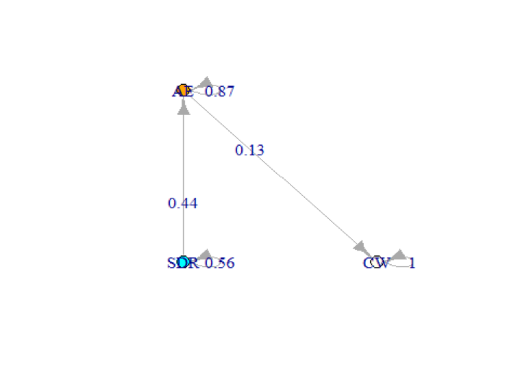
Once that was verified, we plotted the Markov chain structure along with the transition probabilities that were derived from our data. This code instantiates a Markov chain object by defining the transition matrix as well as the names of the states. It also displays the Markov chain and the transition probabilities.

source('TransProb.R')
source('MatDataBase.R')
source('GatherTransMat.R')
transElec <- GatherTransMat('Manufacturing','Between 100M and 500M', 'Between 500 and 1k')

print(transElec)

markov2 <- new('markovchain',
              transitionMatrix = transElec, # These are the transition probabilities of a random industry
              states = c('SDR','AE','CW'))

layout <- matrix(c(0,0,0,1,1,0), ncol = 2, byrow = TRUE)
plot(markov2, node.size = 10, layout = layout)

##           [,1]      [,2]      [,3]
## [1,] 0.5573215 0.4426785 0.0000000
## [2,] 0.0000000 0.8678118 0.1321882
## [3,] 0.0000000 0.0000000 1.0000000

Since we have an absorbing Markov chain, we calculate the expected time until absorption. The first entry of the vector will output the expected number of steps until closing from the SDR funnel while the second entry will output the expected number if we started from the AE funnel.

# Extract Q from the transition matrix
Q <- transElec[1:2,1:2]
# Generate It
It <- diag(2)
#Calculate fundamental matrix
N <- solve(It-Q)
#Generate column vector of 1s
one <- t(t(c(1,1)))

# Calculate the expected steps by matrix multiplication
expected <- N%*%one
print(expected)

##          [,1]
## [1,] 9.823945
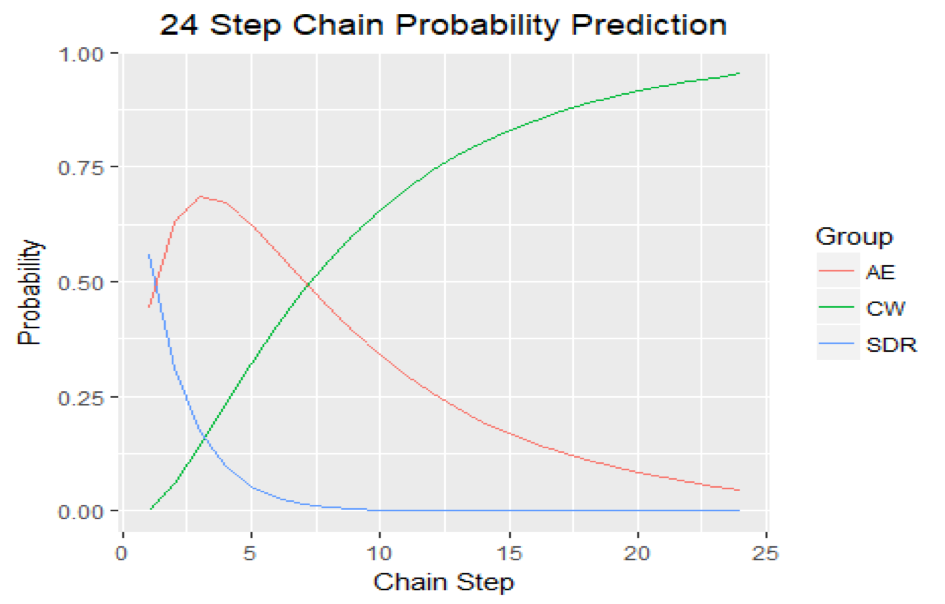
## [2,] 7.564969

However, we can also visualize how the probabilities change as the number of steps increases to contrast the expected number of steps. Thus, we also checked the probabilities of a deal being in any of the three stages for 24 steps.

library(ggplot2)

initState <- c(1,0,0) # The initial state will be SDR Funnel (mimicking setting an initial discovery appointment)

# Initiate probability vectors
SDRProb <- c()
AEProb <- c()
CW <- c()

# Calculate probabilities for 24 steps.
for(k in 1:24){
  nsteps <- initState*markov2^k
  SDRProb[k] <- nsteps[1,1]
  AEProb[k] <- nsteps[1,2]
  CW[k] <- nsteps[1,3]
}

# Make dataframes and merge them
SDRProb <- as.data.frame(SDRProb)
SDRProb$Group <- 'SDR'
SDRProb$Iter <- 1:24
names(SDRProb)[1] <- 'Value'

AEProb <- as.data.frame(AEProb)
AEProb$Group <- 'AE'
AEProb$Iter <- 1:24
names(AEProb)[1] <- 'Value'

CW <- as.data.frame(CW)
CW$Group <- 'CW'
CW$Iter <- 1:24
names(CW)[1] <- 'Value'

steps <- rbind(SDRProb,AEProb,CW)

# Plot the probabilities using ggplot
ggplot(steps, aes(x = Iter, y = Value, col = Group))+
  geom_line() +
  xlab('Chain Step') +
  ylab('Probability') +
  ggtitle('24 Step Chain Probability Prediction')+
  theme(plot.title = element_text(hjust = 0.5))

If we combine both results, it seems apparent that the CW state becomes the most likely state after 6-9 steps. Given that the transition porbabilities are monthly transition probabilities, you can argue that the typical sales velocity from initial appointment set to successfully closing a deal for that industry can be between 6 and 9 months. That's quite a lengthy sales process.

Conclusion

The goal of this analysis was to show how can the basic principles of Markov chains and absorbing Markov chains could be used to answer a question relevant to business. In this case, the Markov chain results were quite accurate despite the time-homogeneous assumptions since further empirical analyses revealed that the average sales velocity for industry used in this analysis was 208 days, which is almost 7 months. Hopefully, this example will serve for you to further explore Markov chains on your own and apply them to your business questions.

If you are interested in learning more about R, take DataCamp's Intermediate R course.

Check out our Markov Chains in Python: Beginner Tutorial.