Course
Introduction to Python
4 hr
6.9M
Run and edit the code from this tutorial online
Run codeA Markov chain is a mathematical system usually defined as a collection of random variables, that transition from one state to another according to certain probabilistic rules. These set of transition satisfies the Markov Property, which states that the probability of transitioning to any particular state is dependent solely on the current state and time elapsed, and not on the sequence of state that preceded it. This unique characteristic of Markov processes render them memoryless.
Want to tackle more statistics topics with Python? Check out DataCamp's Statistical Thinking in Python course!
Let's transition...
Markov Chains have prolific usage in mathematics. They are widely employed in economics, game theory, communication theory, genetics and finance. They arise broadly in statistical specially Bayesian statistics and information-theoretical contexts. When it comes real-world problems, they are used to postulate solutions to study cruise control systems in motor vehicles, queues or lines of customers arriving at an airport, exchange rates of currencies, etc. The algorithm known as PageRank, which was originally proposed for the internet search engine Google, is based on a Markov process. Reddit's Subreddit Simulator is a fully-automated subreddit that generates random submissions and comments using markov chains, so cool!
A Markov chain is a random process with the Markov property. A random process or often called stochastic property is a mathematical object defined as a collection of random variables. A Markov chain has either discrete state space (set of possible values of the random variables) or discrete index set (often representing time) - given the fact, many variations for a Markov chain exists. Usually the term "Markov chain" is reserved for a process with a discrete set of times, that is a Discrete Time Markov chain (DTMC).
A discrete-time Markov chain involves a system which is in a certain state at each step, with the state changing randomly between steps. The steps are often thought of as moments in time (But you might as well refer to physical distance or any other discrete measurement). A discrete time Markov chain is a sequence of random variables X1, X2, X3, ... with the Markov property, such that the probability of moving to the next state depends only on the present state and not on the previous states. Putting this is mathematical probabilistic formula:
Pr( Xn+1 = x | X1 = x1, X2 = x2, …, Xn = xn) = Pr( Xn+1 = x | Xn = xn)
As you can see, the probability of Xn+1 only depends on the probability of Xn that precedes it. Which means the knowledge of the previous state is all that is necessary to determine the probability distribution of the current state, satisfying the rule of conditional independence (or said other way: you only need to know the current state to determine the next state).
The possible values of Xi form a countable set S called the state space of the chain. The state space can be anything: letters, numbers, basketball scores or weather conditions. While the time parameter is usually discrete, the state space of a discrete time Markov chain does not have any widely agreed upon restrictions, and rather refers to a process on an arbitrary state space. However, many applications of Markov chains employ finite or countably infinite state spaces, because they have a more straightforward statistical analysis.
A Markov chain is represented using a probabilistic automaton (It only sounds complicated!). The changes of state of the system are called transitions. The probabilities associated with various state changes are called transition probabilities. A probabilistic automaton includes the probability of a given transition into the transition function, turning it into a transition matrix.
You can think of it as a sequence of directed graphs, where the edges of graph n are labeled by the probabilities of going from one state at time n to the other states at time n+1, Pr(Xn+1 = x | Xn = xn). You can read this as, probability of going to state Xn+1 given value of state Xn. The same information is represented by the transition matrix from time n to time n+1. Every state in the state space is included once as a row and again as a column, and each cell in the matrix tells you the probability of transitioning from its row's state to its column's state.
If the Markov chain has N possible states, the matrix will be an N x N matrix, such that entry (I, J) is the probability of transitioning from state I to state J. Additionally, the transition matrix must be a stochastic matrix, a matrix whose entries in each row must add up to exactly 1. Why? Since each row represents its own probability distribution.
So, the model is characterized by a state space, a transition matrix describing the probabilities of particular transitions, and an initial state across the state space, given in the initial distribution.
Whole lot of words eh?
Let's check out a simple example to understand the concepts:
When Cj is sad, which isn't very usual: she either goes for a run, goobles down icecream or takes a nap.
From historic data, if she spent sleeping a sad day away. The next day it is 60% likely she will go for a run, 20% she will stay in bed the next day and 20% chance she will pig out on icecream.
When she is sad and goes for a run, there is a 60% chances she'll go for a run the next day, 30% she gorges on icecream and only 10% chances she'll spend sleeping the next day.
Finally, when she indulges on icecream on a sad day, there is a mere 10% chance she continues to have icecream the next day as well, 70% she is likely to go for a run and 20% chance that she spends sleeping the next day.
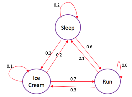
The Markov Chain depicted in the state diagram has 3 possible states: sleep, run, icecream. So, the transition matrix will be 3 x 3 matrix. Notice, the arrows exiting a state always sums up to exactly 1, similarly the entries in each row in the transition matrix must add up to exactly 1 - representing probability distribution. In the transition matrix, the cells do the same job that the arrows do in the state diagram.
Now that you have seen the example, this should give you an idea of the different concepts related to a Markov chain. But, how and where can you use these theory in real life?
With the example that you have seen, you can now answer questions like: "Starting from the state: sleep, what is the probability that Cj will be running (state: run) at the end of a sad 2-day duration?"
Let's work this one out: In order to move from state: sleep to state: run, Cj must either stay on state: sleep the first move (or day), then move to state: run the next (second) move (0.2 $\cdot$ 0.6); or move to state: run the first day and then stay there the second (0.6 $\cdot$ 0.6) or she could transition to state: icecream on the first move and then to state: run in the second (0.2 $\cdot$ 0.7). So the probability: ((0.2 $\cdot$ 0.6) + (0.6 $\cdot$ 0.6) + (0.2 $\cdot$ 0.7)) = 0.62. So, we can now say that there is a 62% chance that Cj will move to state: run after two days of being sad, if she started out in the state: sleep.
Hopefully, this gave you an idea of the various questions you can answer using a Markov Chain network.
Also, with this clear in mind, it becomes easier to understand some important properties of Markov chains:
Tip: if you want to also see a visual explanation of Markov chains, make sure to visit this page.
Let's try to code the example above in Python. And although in real life, you would probably use a library that encodes Markov Chains in a much efficient manner, the code should help you get started...
Let's first import some of the libraries you will use.
import numpy as np
import random as rm
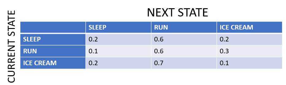
Let's now define the states and their probability: the transition matrix. Remember, the matrix is going to be a 3 X 3 matrix since you have three states. Also, you will have to define the transition paths, you can do this using matrices as well.
# The statespace
states = ["Sleep","Icecream","Run"]

# Possible sequences of events
transitionName = [["SS","SR","SI"],["RS","RR","RI"],["IS","IR","II"]]

# Probabilities matrix (transition matrix)
transitionMatrix = [[0.2,0.6,0.2],[0.1,0.6,0.3],[0.2,0.7,0.1]]
Oh, always make sure the probabilities sum up to 1. And it doesn't hurt to leave error messages, at least when coding!
if sum(transitionMatrix[0])+sum(transitionMatrix[1])+sum(transitionMatrix[1]) != 3:
    print("Somewhere, something went wrong. Transition matrix, perhaps?")
else: print("All is gonna be okay, you should move on!! ;)")
All is gonna be okay, you should move on!! ;)
Now let's code the real thing. You will use the numpy.random.choice to generate a random sample from the set of transitions possible. While most of its arguments are self-explanatory, the p might not be. It is an optional argument that lets you enter the probability distribution for the sampling set, which is the transition matrix in this case.
# A function that implements the Markov model to forecast the state/mood.
def activity_forecast(days):
    # Choose the starting state
    activityToday = "Sleep"
    print("Start state: " + activityToday)
    # Shall store the sequence of states taken. So, this only has the starting state for now.
    activityList = [activityToday]
    i = 0
    # To calculate the probability of the activityList
    prob = 1
    while i != days:
        if activityToday == "Sleep":
            change = np.random.choice(transitionName[0],replace=True,p=transitionMatrix[0])
            if change == "SS":
                prob = prob * 0.2
                activityList.append("Sleep")
                pass
            elif change == "SR":
                prob = prob * 0.6
                activityToday = "Run"
                activityList.append("Run")
            else:
                prob = prob * 0.2
                activityToday = "Icecream"
                activityList.append("Icecream")
        elif activityToday == "Run":
            change = np.random.choice(transitionName[1],replace=True,p=transitionMatrix[1])
            if change == "RR":
                prob = prob * 0.5
                activityList.append("Run")
                pass
            elif change == "RS":
                prob = prob * 0.2
                activityToday = "Sleep"
                activityList.append("Sleep")
            else:
                prob = prob * 0.3
                activityToday = "Icecream"
                activityList.append("Icecream")
        elif activityToday == "Icecream":
            change = np.random.choice(transitionName[2],replace=True,p=transitionMatrix[2])
            if change == "II":
                prob = prob * 0.1
                activityList.append("Icecream")
                pass
            elif change == "IS":
                prob = prob * 0.2
                activityToday = "Sleep"
                activityList.append("Sleep")
            else:
                prob = prob * 0.7
                activityToday = "Run"
                activityList.append("Run")
        i += 1
    print("Possible states: " + str(activityList))
    print("End state after "+ str(days) + " days: " + activityToday)
    print("Probability of the possible sequence of states: " + str(prob))

# Function that forecasts the possible state for the next 2 days
activity_forecast(2)
Start state: Sleep
Possible states: ['Sleep', 'Sleep', 'Run']
End state after 2 days: Run
Probability of the possible sequence of states: 0.12
You get a random set of transitions possible along with the probability of it happening, starting from state: Sleep. Extend the program further to maybe iterate it for a couple of hundred times with the same starting state, you can then see the expected probability of ending at any particular state along with its probability. Let's rewrite the function activity_forecast and add a fresh set of loops to do this...
def activity_forecast(days):
    # Choose the starting state
    activityToday = "Sleep"
    activityList = [activityToday]
    i = 0
    prob = 1
    while i != days:
        if activityToday == "Sleep":
            change = np.random.choice(transitionName[0],replace=True,p=transitionMatrix[0])
            if change == "SS":
                prob = prob * 0.2
                activityList.append("Sleep")
                pass
            elif change == "SR":
                prob = prob * 0.6
                activityToday = "Run"
                activityList.append("Run")
            else:
                prob = prob * 0.2
                activityToday = "Icecream"
                activityList.append("Icecream")
        elif activityToday == "Run":
            change = np.random.choice(transitionName[1],replace=True,p=transitionMatrix[1])
            if change == "RR":
                prob = prob * 0.5
                activityList.append("Run")
                pass
            elif change == "RS":
                prob = prob * 0.2
                activityToday = "Sleep"
                activityList.append("Sleep")
            else:
                prob = prob * 0.3
                activityToday = "Icecream"
                activityList.append("Icecream")
        elif activityToday == "Icecream":
            change = np.random.choice(transitionName[2],replace=True,p=transitionMatrix[2])
            if change == "II":
                prob = prob * 0.1
                activityList.append("Icecream")
                pass
            elif change == "IS":
                prob = prob * 0.2
                activityToday = "Sleep"
                activityList.append("Sleep")
            else:
                prob = prob * 0.7
                activityToday = "Run"
                activityList.append("Run")
        i += 1
    return activityList

# To save every activityList
list_activity = []
count = 0

# `Range` starts from the first count up until but excluding the last count
for iterations in range(1,10000):
        list_activity.append(activity_forecast(2))

# Check out all the `activityList` we collected
#print(list_activity)

# Iterate through the list to get a count of all activities ending in state:'Run'
for smaller_list in list_activity:
    if(smaller_list[2] == "Run"):
        count += 1

# Calculate the probability of starting from state:'Sleep' and ending at state:'Run'
percentage = (count/10000) * 100
print("The probability of starting at state:'Sleep' and ending at state:'Run'= " + str(percentage) + "%")
The probability of starting at state:'Sleep' and ending at state:'Run'= 62.419999999999995%
How did we approximate towards the desired 62%?
Note This is actually the "law of large numbers", which is a principle of probability that states that the frequencies of events with the same likelihood of occurrence even out, but only if there are enough trials or instances. In other words, as the number of experiments increases, the actual ratio of outcomes will converge on a theoretical or expected ratio of outcomes.
This concludes the tutorial on Markov Chains. You have been introduced to Markov Chains and seen some of its properties. Simple Markov chains are one of the required, foundational topics to get started with data science in Python. If you'd like more resources to get started with statistics in Python, make sure to check out this page.
Are you interested in exploring more practical case studies with statistics in Python? Check out DataCamp's Case Studies in Statistical Thinking or Network Analysis in Python courses.
Python Courses
Course
Course
Course
Tutorial
Francisco Javier Carrera Arias
Tutorial
Avinash Navlani
Tutorial
Vidhi Chugh
Tutorial
DataCamp Team
Tutorial
Matthew Przybyla