Time Series Analysis with Spreadsheets Tutorial

ACF and PCF

As the name suggests, Autocorrelation is the linear dependence of a variable with itself at two different data points in time. This function is used to determine how well the present value of the series is related to its past values. ACF takes into consideration all of the components for time series, which are - trends, seasonality, cyclic, and random (residual) while finding correlations. Hence, it’s a complete auto-correlation plot. The ACF is a good way to confirm any positive or negative trend; for a positive trend, you will see the ACF will never be going down.

Another way to determine the linear relationship between any two variables is by partial autocorrelation function. Another way to measure the correlation between two random terms x and xt-1 is to only focus on the portion of correlation, which is explained by xt and xt+1 of and eliminating the linear impact of the random variables that fall in between, xt+1,...., xt+n and then determine the correlation of the transformed random variables. This process is termed as partial autocorrelation function.

Moving Averages

Moving averages smooth the time series data to give a clear indication of where the trend is following. Moving averages help smooth the data by eliminating the noise. For calculating the moving average, you will be taking the arithmetic mean of a variable of the data. There are two types of moving averages, and they are as follows:

• Simple Moving Average: Simple moving average is calculated by taking the arithmetic mean of a given set of values. For example, to calculate a basic 5-day moving average of closing prices, you would add up the closing prices from the past 5 days and then divide the result by 5. One of the key functions of the moving average is to determine the trends (Source).

Where, m = 2k+1. That is, the estimate of the trend-cycle at time t is obtained by averaging values of the time series within k periods of t (Source).

Day 1 - 30
Day 2 - 50
Day 3 -100
Day 4 - 40
Day 5 - 35

Simple Moving Average = 30 + 50 +100 + 40 + 35 / 5
= 255/5
= 51

- Exponential Moving Average: The exponential moving average (EMA) is a type of moving average (MA) that gives weight and emphasizes on the latest data points because simple moving averages can be manipulated if there exists a data point with spikes. Thus, the exponential moving average is also known as the exponentially weighted moving average. For example—considering the above data if you want to calculate you would be using the following formula:

For a given series of n, Where N = 5,
EMA = [Last Value in the series - Second last Value ] (2 / n+1) + Second Last Value,
EMA = (35 - 40) (2 / 6) + 40
EMA = 35.33

Moving Average in Spreadsheets

Applying Simple Moving average to Electric Sales data. Let's compute the 3MA or 3-Moving Average:

1. Let’s first plot the data and see the trend.

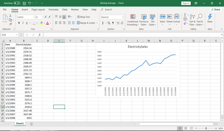
 2. Add a column named Three Moving Average(3MA) and apply the formula. For 3 MA, k value would be -1, 0, 1. You take the average of three terms previous term, current term, and the next term. For the first and last term, 3MA cannot be calculated because there’s no previous term and following term, which we can consider.

 3. We will apply the function in C3,=AVERAGE(B2: B4). This will give the value of 3 MA.

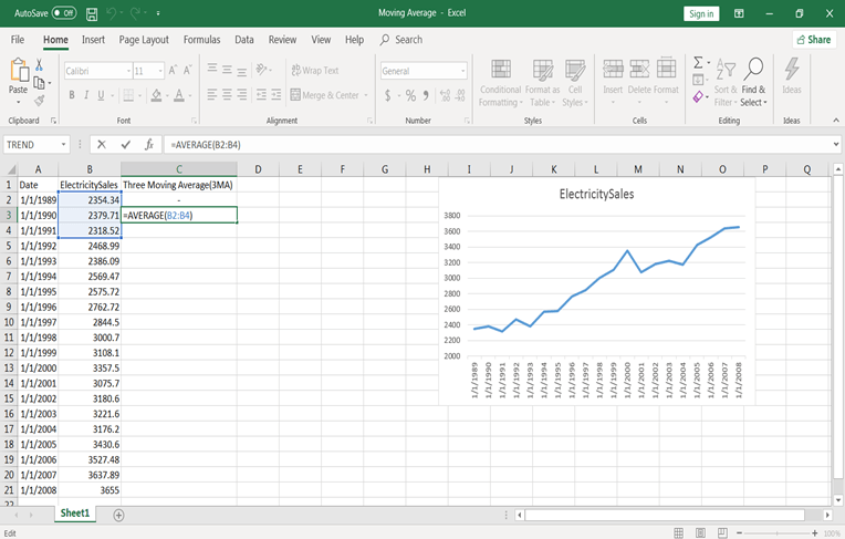
 4. Copy and paste this formula from cell C4 to C20. You will have values.

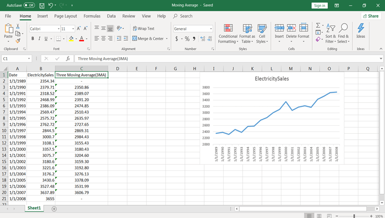
 5. Now select the data and 3MA columns and plot time series. For plotting in the same graph, go to select data and add a series name 3MA. Deselect the 1st and 20th entry because, in 3MA, these values are zero and click on ok.

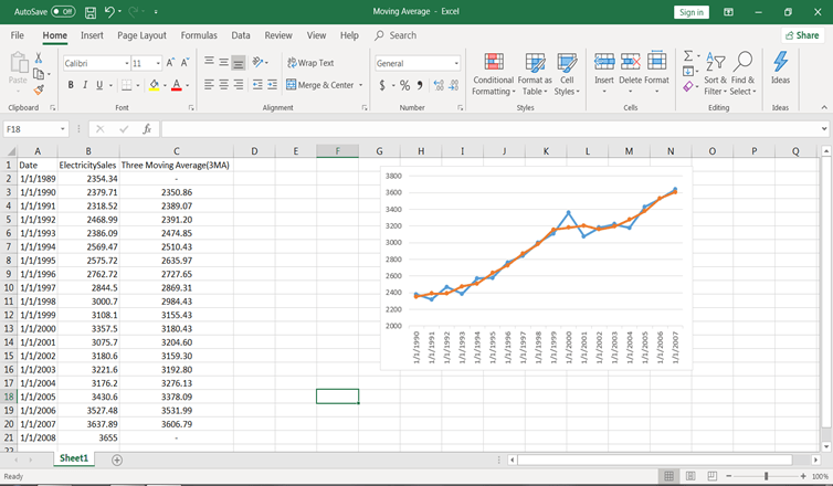
Similarly, you can do for 5 MA, 7MA, etc.

Holt Linear

Until now, you have seen various methods for forecasting, but you can see that these models don’t work well on data with high variations. For instance, if you want to predict the price of bitcoin in the future, which is increasing currently, using the methods stated above wouldn’t be a good option.

If you use any of the above methods, these methods won’t consider the trend. Trend, as discussed earlier, is the component of time series data, that represents the long term movement of a time series. Thus, you require a method that can determine the trend precisely without any assumptions. Hence, you will be using Holt’s Linear Trend method.

Holt’s Linear Method is also known as the Double Exponential Smoothing Technique. This method comprises of three equations which are a forecast equation and two smoothing equations,

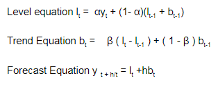
For the first equation, lt is representing the evaluation of the level of time series at time t and bt is representing the evaluation of the slope of the time series at time t.

For the second equation and determining the trend of the current data, first determine the trend of the previous period, by adding bt-1 to the last smoothed value lt-1. This helps to eradicate lag and brings lt to the approximate level of the current data. Since the data can have some randomness or error term in it, in order to eradicate that error, the trend is adjusted by smoothing with β ( lt - lt-1 ), the trend in the last period, and adding that to the previous value of the trend. The last equation is used to forecast the final trend.

Holt Linear in Spreadsheets

Let’s solve this using spreadsheets. You are taking data set from the book “Spyros G. Makridakis, Steven C. Wheelwright, Rob J Hyndman - Forecasting_ Methods and Applications-Wiley (1997)” of holt’s linear method.

1. To initialize the process, you require two estimates—one to get first smoothed values for L1 and the other for the value of trend b1. One alternative is to set L1 = Y1 and b1 = Y2-Y1 or (Y4-Y1)/3.

2. At initial level you considered α = 0.501 and β = 0.072. These you need to optimize. Optimization can be done with MSE (Mean Squared Error) at whatever α and β values you get minimum MSE, consider that as your hyperparameter values.

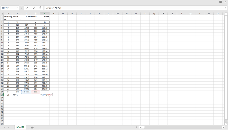
3. Let’s put these formulas into excel to get the forecasted values. At lag 1 (means m = 1) in third equation.

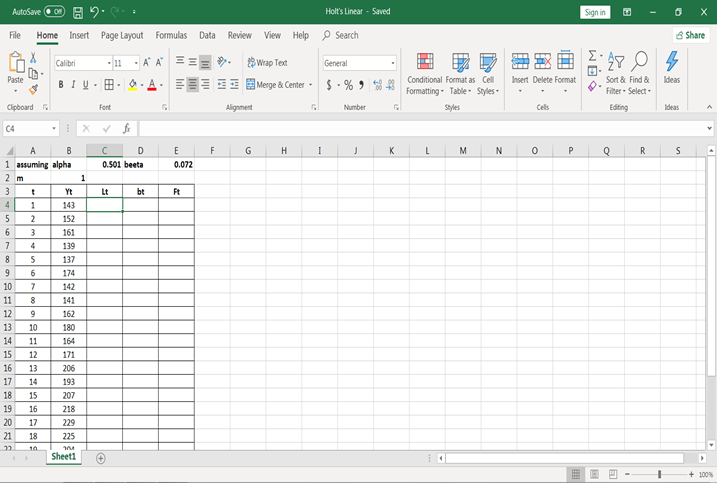
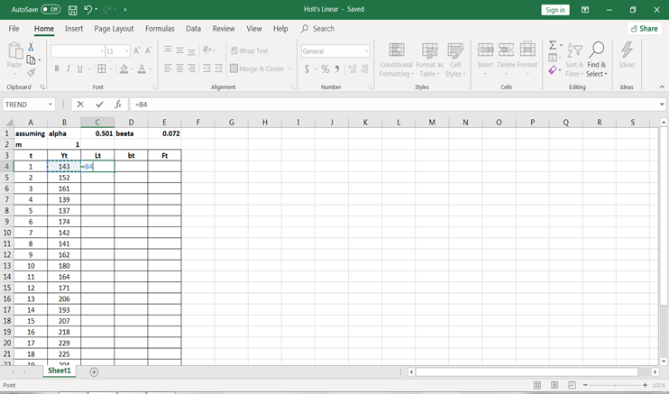
1. As for the initial stage L1 = Y1 and b1 = Y2 – Y1. Let’s assign these values in excel.

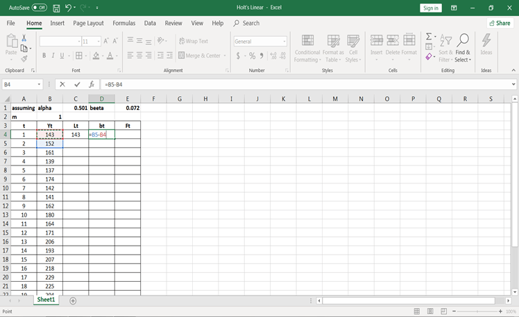
1. Let’s use the formulas to calculate values for L2, b2, and F2.

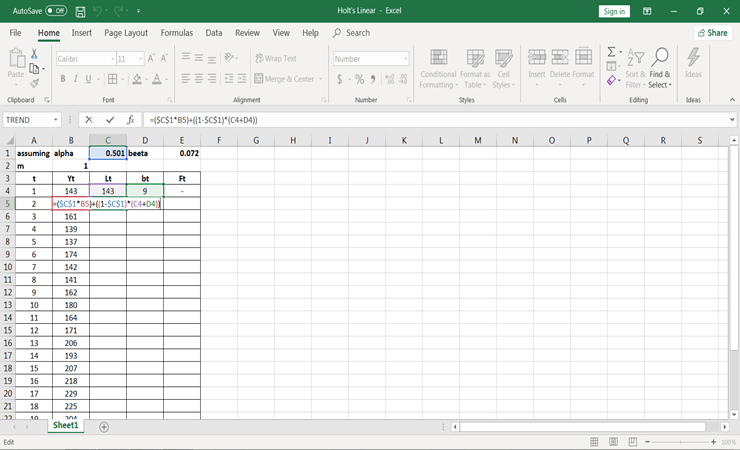
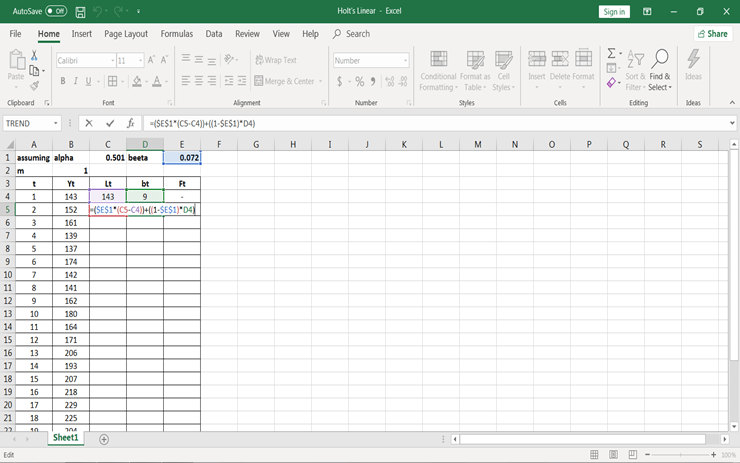
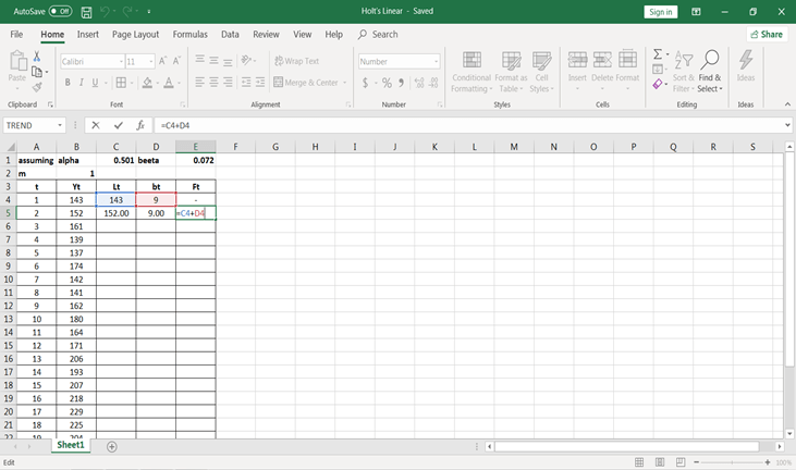
1. Now copy and paste all three formulas till the end of the data available in the file.

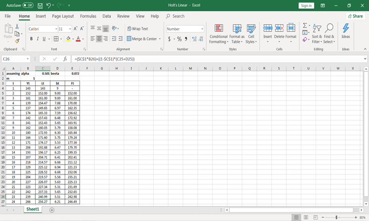
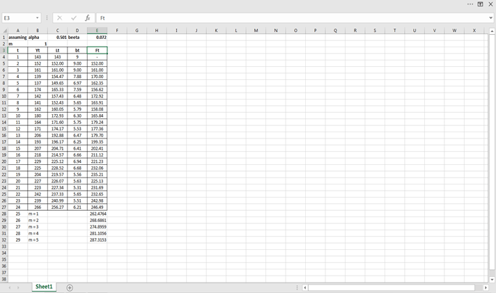
You will have all these values. Now, if you want to forecast for the 25th period, we should consider m = 1 and if for 26th we should consider m = 2 and so on.

1. Let’s calculate forecast values at different periods.

for m = 1,

For m=2,

Similarly, you can calculate at different periods.

Conclusion

Congratulations, you have made it to the end of this tutorial!

In this tutorial, you have covered a lot of details about the time series analysis. You have learned ACF and PCF, moving averages, moving averages in spreadsheets, Holt Linear, and Holt Linear in spreadsheets.

Hopefully, you can now utilize the time series analysis concepts to test the hypothesis. Thanks for reading this tutorial!

If you would like to learn more in spreadsheets, check out DataCamp's Introduction to Statistics in Spreadsheets course.