Top 30 Excel Interview Questions For All Levels

Beginner Excel Interview Questions

These questions are some of the technical Excel interview questions that are relevant to those who are relatively new to the technology. They test the Excel basics, many of which are covered in our Introduction to Excel course.

6. What is an Excel cell reference?

A cell reference in Excel identifies the location of a cell in the spreadsheet. There are two main types of cell references in Excel: absolute and relative.

Relative cell references change relative to the position where they are copied. For example, if you have a formula in cell B2 that references cell A2 (written as =A2), and you copy this formula down to cell B3, the formula in B3 will automatically adjust to reference A3.

Absolute cell references, on the other hand, remain constant no matter where they are copied. They are denoted by the $ symbol in front of the column letter and/or the row number, locking the reference to a specific cell. For instance, if you have a formula in cell B2 referencing cell A2 (=$A$2) and copy this formula to cell B3, the formula will still reference cell A2.

Mixed cell references combine both absolute and relative references. For example, in =A$2, the column reference is relative, and the row reference is absolute. If you copy this formula to the right (to C2), it will change to =B$2, but if you copy it down, it will stay as =A$2.

7. How do you sort data in Excel?

To sort data in Excel, first select the range of cells you want to sort. Click on the Data tab in the ribbon at the top of Excel. Click on the Sort button to open the Sort dialog box. Then, choose Sort A to Z for ascending order or Sort Z to A for descending order if sorting alphabetically. You can also choose to apply custom sorting criteria from the Sort dialog box. Remember to check the My data has headers option if your data includes headers to ensure they are not included in the sorting process.

8. How do you filter data in Excel?

Filtering data in Excel allows you to display only the rows that meet certain criteria. To apply a filter, click on the Data tab, then select Filter – dropdown arrows will be added to each column header. Use these dropdown menus to filter the data.

9. How do you format data in Excel?

In Excel, data formatting is adjusted using the options in the Home tab, where you can change the font type, size, color, cell borders, and background color. For numerical data, right-click a cell or range, select Format Cells, and choose from categories like Number, Currency, Date, or Custom to format the data as desired. Conditional Formatting, also found in the Home tab, allows you to automatically format cells based on their values, such as highlighting cells that contain numbers above a certain threshold.

10. How can you identify duplicates in Excel?

To identify duplicates in a column in Excel, you can use either Conditional Formatting or the COUNTIF() function.

For Conditional Formatting, select the column where you want to identify duplicates, go to the Home tab, click on Conditional Formatting, then Highlight Cell Rules, and choose Duplicate Values. In the dialog box, select how you want the duplicates to be formatted (e.g., with a specific color).

If you choose to use COUNTIF(), enter the formula =COUNTIF(A:A, A1)>1 in a new column adjacent to your data column (assuming your data is in column A), which will return TRUE for duplicate values and FALSE for unique values. Drag the formula down the column to apply it to all cells.

Read our tutorial, How to Highlight Duplicates in Excel, for a more detailed look at both of these methods.

11. How do you remove duplicates in Excel?

One way to remove duplicates in Excel is to first select the range of data or the entire column where you want to remove duplicates. Go to the Data tab on the Ribbon, select Table Tools and click on Remove Duplicates. In the dialog box that appears, specify which columns to check for duplicate information. Click OK, and Excel will remove duplicate rows, keeping only unique records in the selected range. For more detail and to to learn other methods, read our tutorial, How to Remove Duplicates in Excel: 5 Best Methods.

12. How can you freeze panes in Excel?

To freeze panes in Excel, ensure that certain rows or columns remain visible as you scroll through your spreadsheet. First, place your cursor in the cell immediately to the right of the column and below the row you want to freeze. Go to the View tab on the Ribbon, and in the Window group, click on Freeze Panes. From the drop-down menu, select Freeze Panes to freeze the rows above and columns to the left of your selected cell. This feature is particularly useful for keeping headers visible while scrolling through large datasets.

Intermediate Excel Interview Questions

If you’re a more experienced Excel practitioner, you’ll be expected to have more of a grasp of functions and be able to analyze data. Check out our Analysis in Excel course and Intermediate Spreadsheets course to refresh on some of the key points.

13. What's the difference between SUM(), SUMIF(), and SUMIFS()?

In Excel, SUM(), SUMIF(), and SUMIFS() are functions used to calculate the sum of a range of cells, but they differ in their calculation approaches.

The SUM() function simply adds up all the numbers in the specified range. Example: =SUM(A1:A10) will add all the numbers from cells A1 to A10.

SUMIF() adds up cells that meet a single specified criterion. Example: =SUMIF(A1:A10, ">5") will sum all numbers greater than 5 in the range A1 to A10.

SUMIFS() is an extension of SUMIF() and allows for multiple criteria. Example: =SUMIFS(A1:A10, B1:B10, "X", C1:C10, ">5") will sum all numbers in the range A1 to A10 where the corresponding cells in range B1 to B10 equal "X" and those in C1 to C10 are greater than 5.

14. What's the difference between COUNT(), COUNTA(), COUNTBLANK(), and COUNTIF()?

In Excel, COUNT(), COUNTA(), COUNTBLANK(), and COUNTIF() are functions used for counting cells in a range, but each serves a different purpose.

The COUNT() function counts the number of cells in a range that contain numbers. It ignores empty cells, text, or other non-numeric values. Example: =COUNT(A1:A10) will count only the cells in the range A1 to A10 that contain numbers.

COUNTA() counts the number of non-empty cells in a range, regardless of the cell's content (numbers, text, or other types). Example: =COUNTA(A1:A10) will count all cells in the range A1 to A10 that are not empty.

COUNTBLANK() specifically counts the number of empty cells in a given range. Example: =COUNTBLANK(A1:A10) will count the number of empty cells in the range A1 to A10.

COUNTIF() counts the number of cells in a range that meet a specified criterion. Example: =COUNTIF(A1:A10, ">5") will count the number of cells in the range A1 to A10 that contain numbers greater than 5.

15. What's the difference between SUBSTITUTE() and REPLACE()?

​​In Excel, both SUBSTITUTE() and REPLACE() are text functions used to modify string contents, but the string replacement methods are different.

The SUBSTITUTE() function replaces specified occurrences of a text string with another text string.

It is particularly useful when you need to replace specific text within a string and can be used to replace all occurrences or just a specific instance. Example: =SUBSTITUTE("Hello World", "World", "Excel") will change "Hello World" to "Hello Excel". You can also specify which occurrence of "World" to replace if it appears multiple times.

The REPLACE() function, on the other hand, substitutes part of a text string based on its position and the number of characters associated with the string. Example: =REPLACE("Hello World", 7, 5, "Excel") starts at the 7th character (W), replaces 5 characters ("World") with "Excel", also resulting in "Hello Excel".

16. What is a VLOOKUP()? When is it useful?

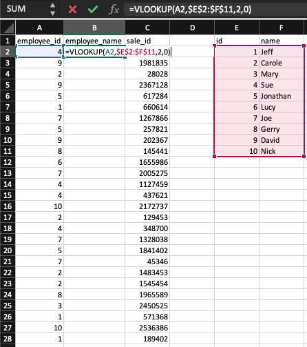
VLOOKUP(), short for vertical lookup, is a function in Excel used for searching for a specific value in one column and retrieving a corresponding value from another column in the same row. It's particularly useful in scenarios where you need to find and extract data from large tables or datasets.

The basic syntax is VLOOKUP(lookup_value, table_array, col_index_num, [range_lookup]), where lookup_value is the value you're searching for, table_array is the range containing the value, col_index_num is the column number in the range containing the return value, and [range_lookup] is an optional argument where TRUE, or 1, finds an approximate match (default) and FALSE, or 0, finds an exact match.

Example: We're interested in returning the employee name (see mapping table E1:F11, where column E stores the employee ID and column F stores the employee name) based on the employee ID found in column A. =VLOOKUP(A2,$E$2:$F$11,2,0) will return "Sue", in the example below.

17. How do you create a PivotTable in Excel?

To create a PivotTable in Excel, first select the data range you want to analyze. Next, go to the Insert tab on the ribbon and click on PivotTable. In the dialog box that appears, choose where you want the PivotTable to be placed (new worksheet or existing worksheet). After clicking OK, the PivotTable Field List pane will appear, where you can drag fields to the different areas (Rows, Columns, Values, and Filters) to organize your data.

18. How do you create a named range?

To create a named range in Excel, first select the cell or range of cells you want to name. Click on the Formulas tab in the ribbon. Then click on Define Name in the Defined Names group. In the New Name dialog box, enter a name for your range in the Name field, and specify the scope and cell reference if needed. Finally, click OK to create the named range.

19. How do you protect a Workbook?

To protect an entire workbook in Excel, navigate to Tools > Protection > Protect Workbook. Enter a password in the dialog box that appears, and then re-enter it when prompted for confirmation. This will encrypt the workbook, requiring the password to open it in the future.

Advanced Excel Interview Questions

This last set of questions is for more advanced users of Excel, those who have a lot of experience using the tool for a variety of purposes.

20. What's the benefit of using INDEX-MATCH instead of VLOOKUP()?

Using INDEX-MATCH in Excel instead of VLOOKUP() offers several advantages: it provides greater flexibility, as it can return a value in a column to the left of the lookup column, unlike VLOOKUP(), which only works left-to-right. INDEX-MATCH is also more efficient in processing, especially for large datasets, as it only looks at specific columns rather than the entire row. It's less prone to errors when columns are added or deleted, since INDEX-MATCH uses column references that don't change with column modifications.

21. How do you create a drop-down list from a data validation?

To create a drop-down list in Excel using data validation, first select the cell or cells where you want the drop-down list to appear. Then, go to the Data tab on the ribbon and click on Validation. In the Data Validation dialog box, under the Settings tab, select List from the Allow: dropdown menu.

In the Source: box, either type in the list items separated by commas, or click the up arrow button to select a range of cells containing the items you want in your list. Ensure that the In-cell dropdown box is checked. Click OK to apply the data validation and create your drop-down list.

22. Can you extract the domain name from an email address?

Assume the email address is example@email.com in cell A1. Enter the following formula in another cell (e.g., B1): =RIGHT(A1, LEN(A1) - FIND("@", A1)), which will yield email.com.

• FIND("@", A1) locates the position of the @ character in the email address.

• LEN(A1) calculates the total length of the email address.

• Subtracting the position of @ from the total length gives us the length of the domain part.

• Finally, RIGHT(A1, LEN(A1) - FIND("@", A1)) extracts the domain part from the right side of the email address.

23. What are wildcards in Excel? How do you apply them?

In Excel, wildcards are special characters used in text searches and functions to represent one or more characters, allowing for more flexible and powerful searching and matching.

The three main wildcards are the asterisk (*), which represents any number of characters, the question mark (?), which represents a single character, and the tilde (~), which is used to escape wildcard characters.

You can use wildcards in various Excel functions like SEARCH, FIND, REPLACE, SUBSTITUTE, and in features like filters or conditional formatting. For example, using =COUNTIF(A1:A10, "*test*") will count all cells in the range A1 to A10 that contain the word "test" anywhere in the text.

24. Can you apply a slicer to filter the data?

To apply a slicer to filter data in Excel, first, ensure your data is formatted as a table or is part of a PivotTable. Click anywhere inside the table or PivotTable, then go to the Insert tab on the Ribbon and click on Slicer in the Filters group. In the dialog box that appears, select the checkbox for the column(s) you want to use for slicing, and then click OK. A slicer will appear in your worksheet, which you can use to filter the data in the table or PivotTable by simply clicking on the various options in the slicer.

25. What is Goal Seek in Excel?

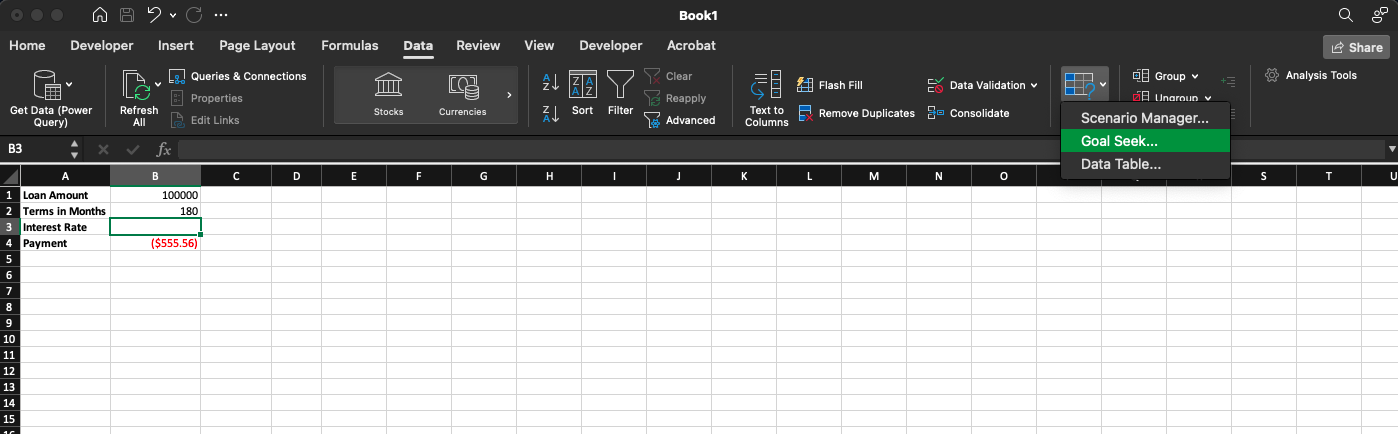
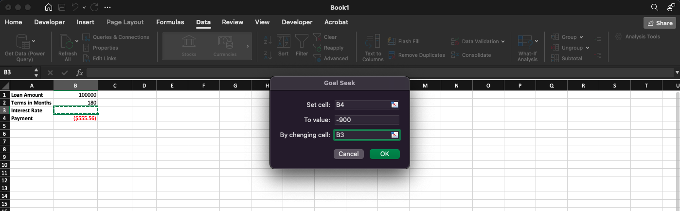
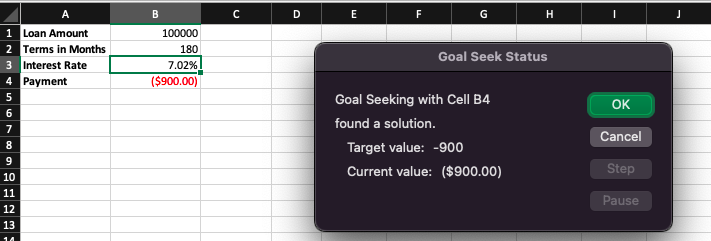
Goal Seek in Excel is a tool that allows you to find the input value needed to achieve a specific goal or target in a formula. It works by adjusting a single input value to make the formula result match the desired outcome. You can access Goal Seek from the Data tab, under the What-If Analysis button, where you specify the cell with the formula, the target value, and the cell to change to achieve this target.

In the example below, we want to know what interest rate we'd pay if we made monthly payments of $900 over a period of 15 years on a $100,000 loan. Goal Seek can help us figure it out!

Excel Interview Questions for Data Analysts

I want to add a final section in case you are interviewing for a data analyst role. Taking our Data Analysis in Excel course is another great way to prepare. 

26. How do you handle missing data in Excel?

To manage missing data in Excel, start by using Conditional Formatting to highlight blank cells. For instance, select your data range, go to Home > Conditional Formatting > Highlight Cell Rules > Blanks, and choose a color. You can replace missing values with averages using the AVERAGE() function. For example, in a new column, use =IF(ISBLANK(A2), AVERAGE($A$2:$A$100), A2) to fill blanks with the column average.

27. Can you explain how to use Excel’s Data Validation feature?

Use Data Validation to limit inputs and maintain data quality. Select the cells where you want restrictions, then go to Data > Data Validation. For instance, to create a dropdown of valid options, choose "List" under "Allow" and type the options separated by commas (e.g., "Yes, No"). This restricts inputs to only these values. You can also use custom formulas, like =ISNUMBER(A1) to ensure only numbers are entered.

28. How do you use Excel’s Power Query for merging datasets?

Power Query makes merging datasets simple. Go to Data > Get Data > Combine Queries > Merge. In the dialog box, select the datasets you want to merge and the common column they share. After loading the data, use Power Query’s transformation tools to clean or shape it. For example, you can filter rows, split columns, or change data types, ensuring consistency in your merged dataset.

29. How do you calculate percentiles or quartiles in Excel?

To calculate percentiles, use the PERCENTILE.INC() or PERCENTILE.EXC() functions. For instance, =PERCENTILE.INC(A1:A100, 0.75) calculates the 75th percentile of the dataset in cells A1:A100. Similarly, to find quartiles, use =QUARTILE(A1:A100, 1) for the first quartile or =QUARTILE(A1:A100, 3) for the third quartile. 

30. Can you describe how to use the Data Analysis Toolpak?

First, enable the Data Analysis Toolpak by going to File > Options > Add-ins > Analysis Toolpak > Manage > Go > OK. For regression analysis, go to Data > Data Analysis > Regression, input your dependent and independent variables, and click OK. Excel will generate a detailed output, including coefficients and R-squared values. Use this for tasks like forecasting or hypothesis testing.

Conclusion

Our last tip for your Excel interview is to keep on learning! Tools like Excel adapt to meet the demands of the market (see the introduction of Python in Excel by Anaconda and the integration of LLM-powered Copilot in Excel by Microsoft). While it's unlikely you'll be tested directly on newly released technology, your knowledge of them can give you an edge over other candidates during an interview (as long as you demonstrate the core competencies required for the job first). Good luck!

If you're feeling last-minute jitters before your interview, you can consult our Excel formulas cheat sheet to brush up on key concepts and formulae. In addition, remember that an interview is just a conversation. Treat it like you were meeting an old friend after a long time.