遗传算法：含Python实现的完整指南

想象一下要为卡车优化配送路线。每辆卡车都有许多可能的路线，而您有许多卡车、许多停靠点。可能组合的数量之多令人望而生畏，找到最佳解就像大海捞针。

为了解决这类问题，我们可以借鉴生物学中的一个概念：进化。在生物学中，自然选择推动着进化。大自然要解决的问题，是找到能让生物体生存和繁殖的最优性状组合。它通过让不同的性状组合相互竞争并选出最优组合来实现这一点。

类似地，我们可以用这个思想来创建一种算法，让不同解相互竞争，并通过选择将其“进化”为最佳解。执行此过程的算法称为遗传算法（GA）。

受自然进化启发，GA 能高效探索解空间，即使对于由多个部分组成的复杂问题，也能发现最优或近最优解。通过模拟自然选择的过程，GA 可以让解随时间“进化”，迭代提升性能。

遗传算法的生物学背景

遗传算法的灵感来源于自然选择和遗传学。它们模仿生物体在世代更替中进化以适应环境的方式。理解 GA 背后的基本生物学原理，有助于理解算法的工作机制并更有策略地使用它们。

自然选择

自然选择使得具有更优良性状组合的个体更可能存活和繁殖。随着时间推移，这些有利性状在种群中会变得更常见。

在 GA 的语境中，这一思想体现在选择适应度更高的个体进行繁殖。这样，它们会将其有利性状或“基因”传递给下一代。

基因、交叉与变异

生物体的性状由其基因编码。基因是 DNA 的组成部分，而 DNA 被组织成染色体。

GA 借用了许多相同的概念和术语。问题的潜在解被表示为“染色体”，通常编码为字符串或数组。染色体中的每个元素对应一个基因，用于决定解的某个特定性状。

交叉（或重组）是一种将两个父代染色体的遗传信息部分组合成一个新染色体的遗传操作，这个新染色体兼具双亲的部分信息，然后传给子代。这就是为什么您可能会有母亲的眼睛颜色和父亲的头发颜色的原因之一。

在 GA 中，交叉通过交换父代染色体片段来创建新个体。该操作引入变异性，并允许子代同时继承双亲的有益性状。

变异会在生物的基因中引入随机变化，从而产生新的性状。

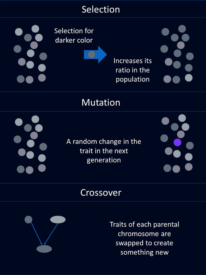
在遗传算法中，变异是随机改变染色体中的一个或多个基因。这有助于在种群内保持遗传多样性，并使算法能够探索解空间的新区域。

适应度评估

在自然界中，个体的适应度由其生存和繁殖的能力决定。如果在繁殖前死亡，适应度就是零。如果您有 12 个孙辈，您的适应度会高于只有 2 个孙辈的人。

在 GA 中，适应度的含义类似但略有不同。适应度函数用于评估某个解在解决当前问题上的表现。适应度更高的解更可能被选中去繁殖，从而确保更好的解在世代间传播。

遗传算法的组成

遗传算法受进化启发。因此，GA 的组成部分在名称和功能上与其生物学对应物相似。这些组件通常各自实现为一个函数。

种群

遗传算法中的种群是一组候选解，通常称为个体。每个个体由一个染色体表示，可以编码为二进制字符串、数组或其他数据结构。

例如，每条染色体可以表示我们需要优化的函数的一组输入值。或者，每条染色体可以表示配送司机的一条卡车路线。

适应度函数

适应度函数用于评估每个个体解决我们关心问题的能力。它为每个个体分配一个适应度值，值越高表示解越好。适应度函数引导算法朝更好的解前进。

例如，在数学函数优化的示例中，适应度函数可能返回给定输入下函数的取值。对于卡车路线示例，适应度函数可能返回完成配送的速度。

选择函数

选择函数基于适应度从种群中挑选个体进行繁殖。适应度更高的个体更可能被选中。这模拟了自然选择，即最适应的个体更可能存活并繁殖。

选择方法有多种。常见方法包括轮盘赌选择、锦标赛选择和基于排序的选择。

轮盘赌选择是指根据与适应度成比例的概率来选择个体，类似于转动轮盘。

锦标赛选择是随机选取一个个体子集，从中选出适应度最高的个体。

基于排序的选择会先按适应度对个体排序，再基于这些排名而非原始适应度值分配选择概率。

每种方法都有其优势，应根据具体问题需求进行选择。

交叉函数

交叉将两个个体的信息结合以生成子代，目标是同时继承双亲的有益性状。常见的交叉技术包括单点交叉、多点交叉、均匀交叉和混合交叉。

单点交叉是在随机位置选择一个点，在该点处交换双亲的遗传信息，生成两个子代。多点交叉使用多个交换点在父代间交换片段，从而形成更复杂的遗传组合。

均匀交叉会随机决定每个基因由哪位父母贡献，提供较高的遗传多样性。混合交叉通过使用随机混合因子来融合父母的基因以生成子代。选择哪种技术应基于问题复杂度以及对子代多样性的期望水平。

变异函数

变异在子代的遗传物质中引入随机变化。这有助于保持种群多样性并探索解空间的新区域。变异可以简单到翻转二进制字符串中的某一位，或根据编码方案涉及更复杂的改变。

遗传算法的执行流程

遗传算法通过一系列模拟自然进化过程的步骤来寻找最优解。这些步骤使种群在世代更替中进化，从而提升解的质量。以下是遗传算法的一般流程：

步骤 1：初始化

首先，我们生成一个初始的随机个体种群。此步骤为算法提供一个多样化的潜在解集合作为起点。

步骤 2：评估

接下来，我们需要计算种群中每个个体的适应度。在这里，我们使用适应度函数来评估每个解的好坏。

步骤 3：选择

根据选择标准，按适应度选择用于繁殖的个体。此步骤决定哪些个体将成为父母。

步骤 4：交叉

然后进行交叉。通过组合被选父母的遗传信息，我们应用交叉技术来生成新解（子代）。

步骤 5：变异

为保持种群多样性，我们需要在子代中引入随机变异。

步骤 6：替换

接着，我们将部分或全部旧种群替换为新的子代，决定哪些个体进入下一代。

步骤 7：重复

将前述步骤 2-6 循环执行指定的代数，或直到满足终止条件为止。通过该循环，种群会随时间进化，理想情况下得到一个良好的解。

Python 示例

既然我们已经了解了遗传算法是什么以及它们的大致工作原理，让我们构建一个遗传算法来解决一个简单的优化问题。

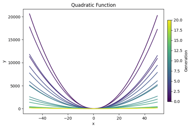
方程 y=ax2+bx+c在图上会形成一条抛物线。我们将使用遗传算法来找到 a、b 和 c 的取值组合，使抛物线尽可能“平”。下面是我们将实现的效果预览：

导入库

在函数的开头，我们将导入必要的库。我们会使用“random”为初始种群生成随机值。Numpy 在进行任何数学计算时通常都很有用（在我看来）。

此外，我坚信应当始终绘制图表来确认代码确实按预期运行。所以我们将导入“matplotlib.pyplot”来绘制图形。

我也喜欢在每一代（假设代数较少）打印出重要结果，以更好地理解仿真过程中的情况。因此，我们会为此导入“PrettyTable”。

import random
import matplotlib.pyplot as plt
import numpy as np
from prettytable import PrettyTable技术支持

定义适应度函数

接下来我们需要定义适应度函数，用于评估每个解的适应度。在这个例子中，我们要找到图上最“平”的 U 形。因此我计算了顶点处的 y 值，以及在 x=-1 与 x=1 处的 y 值。

然后我将这三点处 y 值之间的差值之和作为曲率的度量。由于我们希望得到最平的曲线，我对曲率取了相反数，完成适应度函数。

# Define the fitness function (objective is to create the flattest U-shape)
def fitness_function(params):
    a, b, c = params
    if a <= 0:
        return -float('inf')  # Penalize downward facing u-shapes heavily
    vertex_x = -b / (2 * a) #x value at vertex
    vertex_y = a * (vertex_x ** 2) + b * vertex_x + c #y value at vertex
    y_left = a * (-1) ** 2 + b * (-1) + c #y-coordinate at x = -1
    y_right = a * (1) ** 2 + b * (1) + c #y-coordinate at x = 1
    curviness = abs(y_left - vertex_y) + abs(y_right - vertex_y)
    return -curviness  # Negate to minimize curviness技术支持

创建初始种群

我们将使用“random”库生成一组随机解作为种群。种群中的每个个体都是 a、b 和 c 的一组取值。

# Create the initial population
def create_initial_population(size, lower_bound, upper_bound):
    population = []
    for _ in range(size):
        individual = (random.uniform(lower_bound, upper_bound),
                      random.uniform(lower_bound, upper_bound),
                      random.uniform(lower_bound, upper_bound))
        population.append(individual)
    return population技术支持

创建选择函数

选择函数将决定哪些个体进行繁殖以创建下一代。在本例中，我们将采用锦标赛选择：从种群中随机抽取一个子集，选择其中适应度最高的个体进行繁殖。

# Selection function using tournament selection
def selection(population, fitnesses, tournament_size=3):
    selected = []
    for _ in range(len(population)):
        tournament = random.sample(list(zip(population, fitnesses)), tournament_size)
        winner = max(tournament, key=lambda x: x[1])[0]
        selected.append(winner)
    return selected技术支持

编写交叉函数

接下来，我们将写一个小函数，用交叉根据现有解创建新解。

# Crossover function
def crossover(parent1, parent2):
    alpha = random.random()
    child1 = tuple(alpha * p1 + (1 - alpha) * p2 for p1, p2 in zip(parent1, parent2))
    child2 = tuple(alpha * p2 + (1 - alpha) * p1 for p1, p2 in zip(parent1, parent2))
    return child1, child2技术支持

设计变异函数

我们还需要一个变异函数，为后续世代引入随机性。这对于确保每一代都有足够的多样性可供选择非常重要。

# Mutation function
def mutation(individual, mutation_rate, lower_bound, upper_bound):
    individual = list(individual)
    for i in range(len(individual)):
        if random.random() < mutation_rate:
            mutation_amount = random.uniform(-1, 1)
            individual[i] += mutation_amount
            # Ensure the individual stays within bounds
            individual[i] = max(min(individual[i], upper_bound), lower_bound)
    return tuple(individual)技术支持

主循环

接下来我们需要创建主循环，将这些部分组合起来运行算法。由于还需要绘图，我会在本节加入绘图代码，以及生成最终表格所需的代码。

# Main genetic algorithm function
def genetic_algorithm(population_size, lower_bound, upper_bound, generations, mutation_rate):
    population = create_initial_population(population_size, lower_bound, upper_bound)
    
    # Prepare for plotting
    fig, axs = plt.subplots(3, 1, figsize=(12, 18))  # 3 rows, 1 column for subplots
    best_performers = []
    all_populations = []

    # Prepare for table
    table = PrettyTable()
    table.field_names = ["Generation", "a", "b", "c", "Fitness"]

    for generation in range(generations):
        fitnesses = [fitness_function(ind) for ind in population]

        # Store the best performer of the current generation
        best_individual = max(population, key=fitness_function)
        best_fitness = fitness_function(best_individual)
        best_performers.append((best_individual, best_fitness))
        all_populations.append(population[:])
        table.add_row([generation + 1, best_individual[0], best_individual[1], best_individual[2], best_fitness])

        population = selection(population, fitnesses)

        next_population = []
        for i in range(0, len(population), 2):
            parent1 = population[i]
            parent2 = population[i + 1]

            child1, child2 = crossover(parent1, parent2)

            next_population.append(mutation(child1, mutation_rate, lower_bound, upper_bound))
            next_population.append(mutation(child2, mutation_rate, lower_bound, upper_bound))

        # Replace the old population with the new one, preserving the best individual
        next_population[0] = best_individual
        population = next_population

    # Print the table
    print(table)

    # Plot the population of one generation (last generation)
    final_population = all_populations[-1]
    final_fitnesses = [fitness_function(ind) for ind in final_population]

    axs[0].scatter(range(len(final_population)), [ind[0] for ind in final_population], color='blue', label='a')
    axs[0].scatter([final_population.index(best_individual)], [best_individual[0]], color='cyan', s=100, label='Best Individual a')
    axs[0].set_ylabel('a', color='blue')
    axs[0].legend(loc='upper left')
    
    axs[1].scatter(range(len(final_population)), [ind[1] for ind in final_population], color='green', label='b')
    axs[1].scatter([final_population.index(best_individual)], [best_individual[1]], color='magenta', s=100, label='Best Individual b')
    axs[1].set_ylabel('b', color='green')
    axs[1].legend(loc='upper left')
    
    axs[2].scatter(range(len(final_population)), [ind[2] for ind in final_population], color='red', label='c')
    axs[2].scatter([final_population.index(best_individual)], [best_individual[2]], color='yellow', s=100, label='Best Individual c')
    axs[2].set_ylabel('c', color='red')
    axs[2].set_xlabel('Individual Index')
    axs[2].legend(loc='upper left')
    
    axs[0].set_title(f'Final Generation ({generations}) Population Solutions')

    # Plot the values of a, b, and c over generations
    generations_list = range(1, len(best_performers) + 1)
    a_values = [ind[0][0] for ind in best_performers]
    b_values = [ind[0][1] for ind in best_performers]
    c_values = [ind[0][2] for ind in best_performers]
    fig, ax = plt.subplots()
    ax.plot(generations_list, a_values, label='a', color='blue')
    ax.plot(generations_list, b_values, label='b', color='green')
    ax.plot(generations_list, c_values, label='c', color='red')
    ax.set_xlabel('Generation')
    ax.set_ylabel('Parameter Values')
    ax.set_title('Parameter Values Over Generations')
    ax.legend()

    # Plot the fitness values over generations
    best_fitness_values = [fit[1] for fit in best_performers]
    min_fitness_values = [min([fitness_function(ind) for ind in population]) for population in all_populations]
    max_fitness_values = [max([fitness_function(ind) for ind in population]) for population in all_populations]
    fig, ax = plt.subplots()
    ax.plot(generations_list, best_fitness_values, label='Best Fitness', color='black')
    ax.fill_between(generations_list, min_fitness_values, max_fitness_values, color='gray', alpha=0.5, label='Fitness Range')
    ax.set_xlabel('Generation')
    ax.set_ylabel('Fitness')
    ax.set_title('Fitness Over Generations')
    ax.legend()

    # Plot the quadratic function for each generation
    fig, ax = plt.subplots()
    colors = plt.cm.viridis(np.linspace(0, 1, generations))
    for i, (best_ind, best_fit) in enumerate(best_performers):
        color = colors[i]
        a, b, c = best_ind
        x_range = np.linspace(lower_bound, upper_bound, 400)
        y_values = a * (x_range ** 2) + b * x_range + c
        ax.plot(x_range, y_values, color=color)

    ax.set_xlabel('x')
    ax.set_ylabel('y')
    ax.set_title('Quadratic Function')

    # Create a subplot for the colorbar
    cax = fig.add_axes([0.92, 0.2, 0.02, 0.6])  # [left, bottom, width, height]
    norm = plt.cm.colors.Normalize(vmin=0, vmax=generations)
    sm = plt.cm.ScalarMappable(cmap='viridis', norm=norm)
    sm.set_array([])
    fig.colorbar(sm, ax=ax, cax=cax, orientation='vertical', label='Generation')

    plt.show()

    return max(population, key=fitness_function)技术支持

让一切跑起来

最后，我们需要设置算法的参数并运行它。

# Parameters for the genetic algorithm
population_size = 100
lower_bound = -50
upper_bound = 50
generations = 20
mutation_rate = 1

# Run the genetic algorithm
best_solution = genetic_algorithm(population_size, lower_bound, upper_bound, generations, mutation_rate)
print(f"Best solution found: a = {best_solution[0]}, b = {best_solution[1]}, c = {best_solution[2]}")技术支持

终止条件（可选）

在本例中，我们设置了一个固定的代数来运行算法。不过，我们也可以设置一个终止条件：当达到目标适应度时停止程序。大致如下所示：

def termination_condition(fitnesses, target_fitness):
    return max(fitnesses) >= target_fitness技术支持

整合到一起

下面是完整代码的汇总。

import random
import matplotlib.pyplot as plt
import numpy as np
from prettytable import PrettyTable

# Define the fitness function (objective is to create the flattest U-shape)
def fitness_function(params):
    a, b, c = params
    if a <= 0:
        return -float('inf')  # Penalize downward facing u-shapes heavily
    vertex_x = -b / (2 * a) #x value at vertex
    vertex_y = a * (vertex_x ** 2) + b * vertex_x + c #y value at vertex
    y_left = a * (-1) ** 2 + b * (-1) + c #y-coordinate at x = -1
    y_right = a * (1) ** 2 + b * (1) + c #y-coordinate at x = 1
    curviness = abs(y_left - vertex_y) + abs(y_right - vertex_y)
    return -curviness  # Negate to minimize curviness

# Create the initial population
def create_initial_population(size, lower_bound, upper_bound):
    population = []
    for _ in range(size):
        individual = (random.uniform(lower_bound, upper_bound),
                      random.uniform(lower_bound, upper_bound),
                      random.uniform(lower_bound, upper_bound))
        population.append(individual)
    return population

# Selection function using tournament selection
def selection(population, fitnesses, tournament_size=3):
    selected = []
    for _ in range(len(population)):
        tournament = random.sample(list(zip(population, fitnesses)), tournament_size)
        winner = max(tournament, key=lambda x: x[1])[0]
        selected.append(winner)
    return selected

# Crossover function
def crossover(parent1, parent2):
    alpha = random.random()
    child1 = tuple(alpha * p1 + (1 - alpha) * p2 for p1, p2 in zip(parent1, parent2))
    child2 = tuple(alpha * p2 + (1 - alpha) * p1 for p1, p2 in zip(parent1, parent2))
    return child1, child2

# Mutation function
def mutation(individual, mutation_rate, lower_bound, upper_bound):
    individual = list(individual)
    for i in range(len(individual)):
        if random.random() < mutation_rate:
            mutation_amount = random.uniform(-1, 1)
            individual[i] += mutation_amount
            # Ensure the individual stays within bounds
            individual[i] = max(min(individual[i], upper_bound), lower_bound)
    return tuple(individual)

# Main genetic algorithm function
def genetic_algorithm(population_size, lower_bound, upper_bound, generations, mutation_rate):
    population = create_initial_population(population_size, lower_bound, upper_bound)
    
    # Prepare for plotting
    fig, axs = plt.subplots(3, 1, figsize=(12, 18))  # 3 rows, 1 column for subplots
    best_performers = []
    all_populations = []

    # Prepare for table
    table = PrettyTable()
    table.field_names = ["Generation", "a", "b", "c", "Fitness"]

    for generation in range(generations):
        fitnesses = [fitness_function(ind) for ind in population]

        # Store the best performer of the current generation
        best_individual = max(population, key=fitness_function)
        best_fitness = fitness_function(best_individual)
        best_performers.append((best_individual, best_fitness))
        all_populations.append(population[:])
        table.add_row([generation + 1, best_individual[0], best_individual[1], best_individual[2], best_fitness])

        population = selection(population, fitnesses)

        next_population = []
        for i in range(0, len(population), 2):
            parent1 = population[i]
            parent2 = population[i + 1]

            child1, child2 = crossover(parent1, parent2)

            next_population.append(mutation(child1, mutation_rate, lower_bound, upper_bound))
            next_population.append(mutation(child2, mutation_rate, lower_bound, upper_bound))

        # Replace the old population with the new one, preserving the best individual
        next_population[0] = best_individual
        population = next_population

    # Print the table
    print(table)

    # Plot the population of one generation (last generation)
    final_population = all_populations[-1]
    final_fitnesses = [fitness_function(ind) for ind in final_population]

    axs[0].scatter(range(len(final_population)), [ind[0] for ind in final_population], color='blue', label='a')
    axs[0].scatter([final_population.index(best_individual)], [best_individual[0]], color='cyan', s=100, label='Best Individual a')
    axs[0].set_ylabel('a', color='blue')
    axs[0].legend(loc='upper left')
    
    axs[1].scatter(range(len(final_population)), [ind[1] for ind in final_population], color='green', label='b')
    axs[1].scatter([final_population.index(best_individual)], [best_individual[1]], color='magenta', s=100, label='Best Individual b')
    axs[1].set_ylabel('b', color='green')
    axs[1].legend(loc='upper left')
    
    axs[2].scatter(range(len(final_population)), [ind[2] for ind in final_population], color='red', label='c')
    axs[2].scatter([final_population.index(best_individual)], [best_individual[2]], color='yellow', s=100, label='Best Individual c')
    axs[2].set_ylabel('c', color='red')
    axs[2].set_xlabel('Individual Index')
    axs[2].legend(loc='upper left')
    
    axs[0].set_title(f'Final Generation ({generations}) Population Solutions')

    # Plot the values of a, b, and c over generations
    generations_list = range(1, len(best_performers) + 1)
    a_values = [ind[0][0] for ind in best_performers]
    b_values = [ind[0][1] for ind in best_performers]
    c_values = [ind[0][2] for ind in best_performers]
    fig, ax = plt.subplots()
    ax.plot(generations_list, a_values, label='a', color='blue')
    ax.plot(generations_list, b_values, label='b', color='green')
    ax.plot(generations_list, c_values, label='c', color='red')
    ax.set_xlabel('Generation')
    ax.set_ylabel('Parameter Values')
    ax.set_title('Parameter Values Over Generations')
    ax.legend()

    # Plot the fitness values over generations
    best_fitness_values = [fit[1] for fit in best_performers]
    min_fitness_values = [min([fitness_function(ind) for ind in population]) for population in all_populations]
    max_fitness_values = [max([fitness_function(ind) for ind in population]) for population in all_populations]
    fig, ax = plt.subplots()
    ax.plot(generations_list, best_fitness_values, label='Best Fitness', color='black')
    ax.fill_between(generations_list, min_fitness_values, max_fitness_values, color='gray', alpha=0.5, label='Fitness Range')
    ax.set_xlabel('Generation')
    ax.set_ylabel('Fitness')
    ax.set_title('Fitness Over Generations')
    ax.legend()

    # Plot the quadratic function for each generation
    fig, ax = plt.subplots()
    colors = plt.cm.viridis(np.linspace(0, 1, generations))
    for i, (best_ind, best_fit) in enumerate(best_performers):
        color = colors[i]
        a, b, c = best_ind
        x_range = np.linspace(lower_bound, upper_bound, 400)
        y_values = a * (x_range ** 2) + b * x_range + c
        ax.plot(x_range, y_values, color=color)

    ax.set_xlabel('x')
    ax.set_ylabel('y')
    ax.set_title('Quadratic Function')

    # Create a subplot for the colorbar
    cax = fig.add_axes([0.92, 0.2, 0.02, 0.6])  # [left, bottom, width, height]
    norm = plt.cm.colors.Normalize(vmin=0, vmax=generations)
    sm = plt.cm.ScalarMappable(cmap='viridis', norm=norm)
    sm.set_array([])
    fig.colorbar(sm, ax=ax, cax=cax, orientation='vertical', label='Generation')

    plt.show()

    return max(population, key=fitness_function)

# Parameters for the genetic algorithm
population_size = 100
lower_bound = -50
upper_bound = 50
generations = 20
mutation_rate = 1

# Run the genetic algorithm
best_solution = genetic_algorithm(population_size, lower_bound, upper_bound, generations, mutation_rate)
print(f"Best solution found: a = {best_solution[0]}, b = {best_solution[1]}, c = {best_solution[2]}")技术支持

结果评估

让我们利用输出结果来看看我们的函数表现如何。

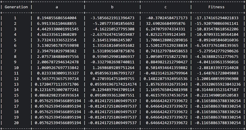
首先，从表格可见我们完成了 20 代，且适应度似乎在每一代中从相对负值逐步提升为不那么负的值。不错！

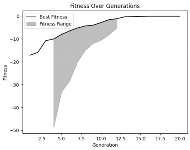
从适应度图中，我们可以确认适应度确实随时间改善，并在后期几代有所趋平。但我们也能看到，在早期几代中出现了一些非常糟糕的解，而我们的模型也正确地将其淘汰。

我们还可以看到，在若干代中适应度范围的多样性并不大。虽然这不一定是坏事，但值得留意。在某些情况下，这可能意味着过早收敛，即当种群缺乏足够多样性时出现的问题。

接下来，让我们绘制每一代的方程，看看是否真的变“平”了。

我们可以看到，早期几代的解曲率较大，这很合理。这个方程会产生 U 形图像。但也能看到，后续世代逐渐变得更平。这正是我们所期望的！

另外需要说明的是，我们明确只在 -50 到 50 的边界内观察。如果把图拉远，即使这些看似平的线也仍是 U 形，只是底部更宽。

这个例子强调了在分析中谨慎对待假设以确保它们支持我们的预期的重要性。我们的模型完全按要求行事，但仅在我们设定的边界内。如果我们想在更远的范围上找到能生成平坦形状的变量组合，就需要在更宽的边界下重新运行模型。

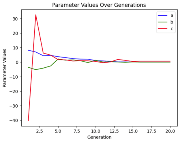
我们可以分别绘制各个变量，观察它们在各代中的变化幅度。可以看到，在本次仿真中，c 在早期波动很大，而 a 和 b 的变化要平缓得多。即便不更改任何参数，每次运行该仿真，该图也会不同，因为初始种群是随机的。

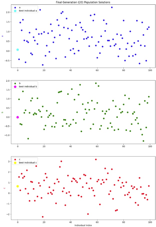
我最后想看的图，是某一代（最终一代）整个种群的快照。由于种群中每个个体有三个参数，我决定将它们拆分成三个子图，而不是折腾三维图。

我真正想从这些图中看到的是这一代内部是否具有良好的多样性。缺乏足够多样性，我们可能会陷入仅有低适应度解可选的局面，从而导致过早收敛。但这些图看起来显示了良好的多样性，因此我对这个结果很满意。

注意事项与建议

遗传算法可用于多种场景。但仍有一些事项需要留意。

参数调优

与任何模型一样，遗传算法的性能取决于多种参数，尤其是种群规模、交叉率、变异率和边界参数。更改这些参数会改变模型的表现。

一般而言，更大的种群规模会帮助您更快找到最优解，因为可选择的方案更多。然而，种群越大，运行所需的时间与资源也越多。

更高的交叉率可以通过更频繁地组合不同个体的有益性状来加速收敛。但交叉率过高可能会破坏种群结构，导致过早收敛。

更高的变异率有助于保持遗传多样性，防止算法陷入局部最优。然而，如果变异率过高，会引入过多随机性，从而干扰收敛过程，使算法难以细化解。

边界参数定义了算法搜索解的范围。应结合具体业务问题进行调优。搜索范围过窄可能错过最优解；范围过宽则会消耗更多时间与资源。当然，还有其他权衡。

例如，在上面的代码示例中，该方程理论上没有界限。但在实践中，我们不可能要求计算机在无限大的图中寻找最平的弧线。因此边界是必要的。但改变这些边界也会改变最优答案。在我看来，为具体用例设定合适的边界对任何模型都至关重要。

您的特定模型中可能还有其他重要参数需要调优。请尝试不同取值，以找到适合您问题的最佳设置。要了解如何专门调优 GA，请参阅 Informed Methods: Genetic Algorithms。

编码

编码是在构建遗传算法时的重要步骤。它涉及将潜在解转换为算法可处理的格式。比如，我们要为卡车优化配送路线。如何把配送地点列表转换为可以放入 GA 的染色体？编码会将这个列表转换为算法可操作的序列，例如表示某条可行配送路线的地点有序列表。

合理的编码能确保遗传算法有效地探索解空间，并以有意义的方式组合或变异解。没有编码，算法将无法处理复杂数据。诸如配送地点、排程问题或客户服务交互等数据，只有通过编码，计算机才能加以利用。

可供选择的编码方案有多种。您可以在以下内容中了解更多，以决定哪种更适合您的情境： Working with Categorical Data in Python 或 How to Convert Strings to Bytes in Python。

过早收敛

过早收敛是指当种群变得过于相似时出现的问题，这会导致算法陷入局部最优而非找到全局最优。实质上，如果种群缺乏足够多样性，解就会“近亲繁殖”，从而无法得到最佳解。

为避免过早收敛，可以尝试几种技术。提高变异率可以引入更多多样性，帮助探索解空间的新区域。您也可以从更具多样性的初始种群开始，确保从一开始就广泛探索解空间。

如果仍然出现过早收敛，您可以尝试根据算法进展动态调整变异率和交叉率。或者，可以使用多个种群（可理解为“岛屿”），并偶尔在它们之间交换个体以维持多样性。

您可以在 Monitoring Machine Learning Concepts 课程中了解更多关于过早收敛和其他机器学习误区的内容。

精英保留

另一方面，较强的交叉与变异或选择中的随机性，可能导致优秀的解没有机会繁殖。这时可以考虑精英保留。精英保留是一种将最佳个体直接保留到下一代以保存优秀解的技术，有助于确保优秀解不会在进化过程中丢失。

然而，使用精英保留时需谨慎。如果没有足够的种群多样性，精英保留可能反而导致过早收敛。如果您的业务问题需要采用精英策略，请确保与足够强的交叉和变异函数以及较大的种群规模配套使用。此方法有助于在利用已知好解与探索新可能性之间保持健康的平衡。

结论

遗传算法是数据科学汲取自然世界灵感的一个绝佳例子。通过模拟自然选择过程，它们为解决复杂的优化问题提供了一种强大的方法。

如果您对其他受生物学启发的模型感兴趣，可以在 Introduction to Deep Learning in Python 中了解神经网络及其他深度学习技术。您或许也会对 DataCamp 的 Generative AI Concepts course 和 AI Ethics 感兴趣。

如果您受到启发想用生物数据做项目，可以查看 Analyzing Genomic Data in R 或 Biomedical Image Analysis in Python。

作者

Amberle McKee

我拥有博士学位，在生物研究环境中从事数据相关工作已有13年。我使用包括 Python、MATLAB 和 R 在内的多种编程语言开发软件。我热衷于与世界分享我对学习的热爱。

主题

数据工程