Genetic Algorithm: Complete Guide With Python Implementation

Inspired by natural evolution, GAs efficiently explore the solution space to discover optimal or near-optimal solutions, even for complex problems with multiple moving parts. By mimicking the process of natural selection, GAs can evolve solutions over time, improving their performance iteratively.

Biological Background of Genetic Algorithms

Genetic algorithms were inspired by the process of natural selection and genetics. They mimic the way living organisms evolve over generations to adapt and survive in their environments. Understanding the basic biological principles behind GAs can help us understand how these algorithms work and help us use them more strategically.

Natural selection

Natural selection is the process that causes individuals with better combinations of favorable traits to be more likely to survive and reproduce. Over time, these advantageous traits become more common in the population.

In the context of GAs, this concept is mirrored by selecting individuals with higher fitness scores for reproduction. In this way, they pass on their favorable traits, or "genes," to the next generation.

Genes, crossover, and mutation

A biological organism's traits are encoded by its genes. Genes are part of DNA, which is arranged into chromosomes.

GAs borrow a lot of the same concepts and terminology. Potential solutions to a problem are represented as "chromosomes," which are typically coded as strings or arrays. Each element in the chromosome corresponds to a gene that determines a specific trait of the solution.

Crossover, or recombination, is a genetic operation that combines parts of the genetic material of two parent chromosomes into a new chromosome that has parts of each parent. This new chromosome mashup is passed on to the child. It’s one reason why you can get your mother’s eye color and your father’s hair color.

In GAs, crossover involves exchanging segments of the parent chromosomes to create new individuals. This operation introduces variability and allows the offspring to inherit beneficial traits from both parents.

Mutation introduces random changes to an organism's genes, which can lead to new traits.

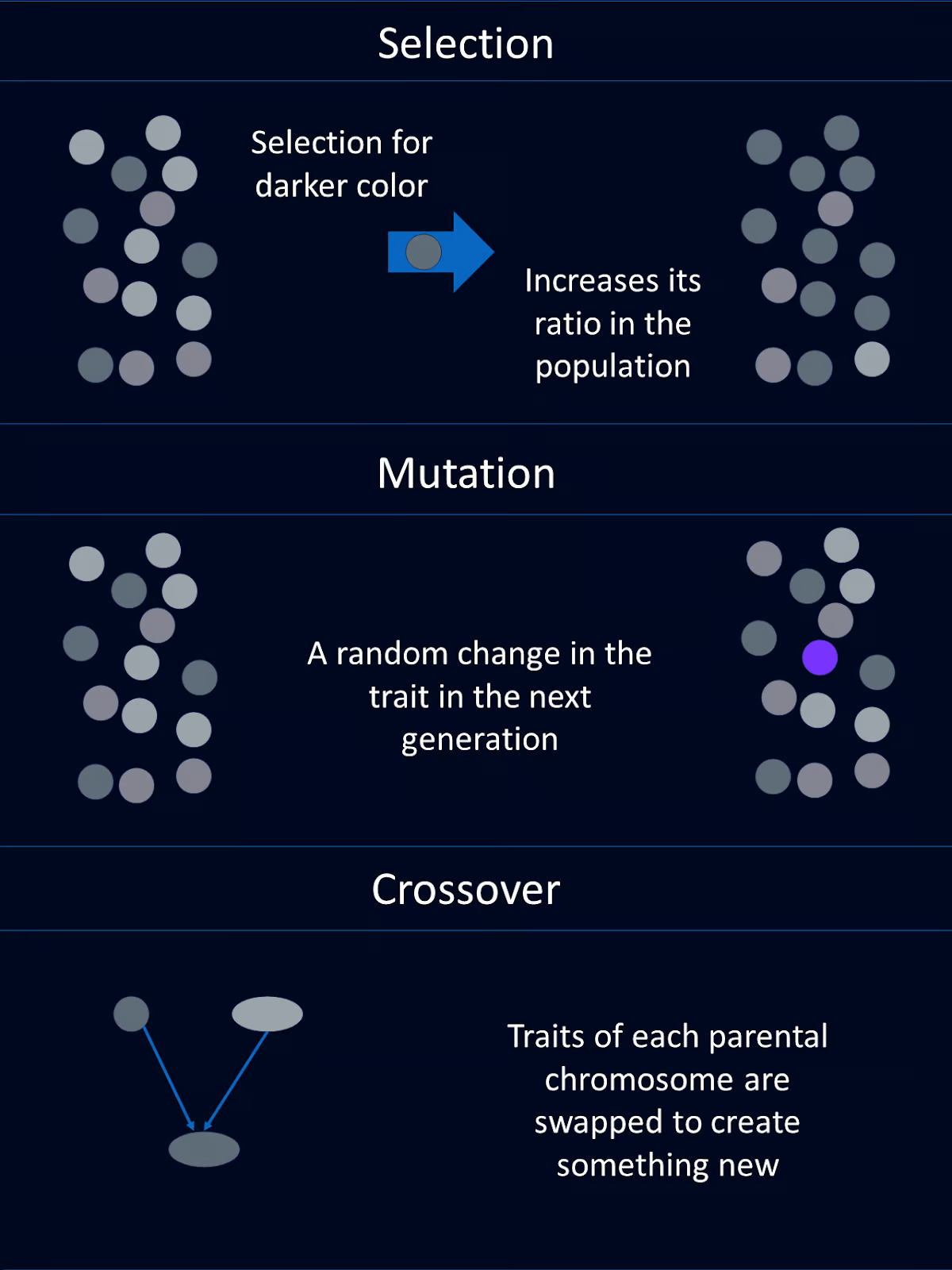
In genetic algorithms, mutation involves randomly altering one or more genes in a chromosome. This helps maintain genetic diversity within the population and allows the algorithm to explore new areas of the solution space.

Fitness evaluation

In nature, an individual's fitness is determined by its ability to survive and reproduce. If you die before you reproduce, you have a fitness of zero. If you have 12 grandchildren your fitness will be higher than someone with 2 grandchildren.

In GAs, fitness is similar, but a little different. A fitness function evaluates how well a solution solves the problem at hand. Solutions with higher fitness scores are more likely to be selected for reproduction, ensuring that better solutions propagate through generations.

Components of a Genetic Algorithm

Genetic algorithms were inspired by evolution. Consequently, the components of a GA share names and functions similar to those of their biological counterparts. Each of these components is usually coded as their own function.

Population

The population in a genetic algorithm is a set of candidate solutions, often called individuals. Each individual is represented as a chromosome, which can be coded as binary strings, arrays, or other data structures.

For example, each chromosome could represent a set of input values to a function we need to optimize. Or each chromosome could represent a truck route for delivery drivers.

Fitness function

The fitness function evaluates each individual's ability to solve the problem we’re interested in. It assigns a fitness value to each individual, with higher values for better solutions. The fitness function guides the algorithm toward better solutions.

For instance, in our mathematical function optimization example, the fitness function might return the value of the function for the given inputs. For our truck routes example, the fitness function might return the speed of delivery completion.

Selection function

The selection function chooses individuals from the population to reproduce based on their fitness. Individuals with higher fitness are more likely to be chosen for reproduction. This mimics natural selection, where the best-adapted individuals are more likely to survive and reproduce.

There are a few different selection methods. Common selection methods include roulette wheel selection, tournament selection, and rank-based selection.

Roulette wheel selection is where individuals are selected based on a probability proportional to their fitness, similar to spinning a roulette wheel.

In tournament selection a subset of individuals is chosen at random and the fittest individual from this subset is selected.

Rank-based selection ranks individuals based on their fitness. Then selection probabilities are assigned based on these ranks rather than raw fitness values.

Each method has its own advantages and should be chosen based on the specific requirements of the problem at hand.

Crossover function

Crossover combines information from two individuals to create offspring. The goal is to inherit beneficial traits from both parents. Common crossover techniques include single-point crossover, multi-point crossover, uniform crossover, and blend crossover.

Single-point crossover involves choosing a random point and swapping the genetic material from two parents at that point to create two offspring. Multi-point crossover uses multiple points for swapping segments between parents, allowing for more complex genetic combinations.

Uniform crossover randomly decides which parent will contribute each gene, providing a high level of genetic diversity. Blend crossover generates offspring by blending the genes of the parents using a random blending factor. The decision of which technique to use should be based on the problem's complexity and the desired level of diversity in the offspring.

Mutation function

Mutation introduces random changes in the offspring's genetic material. This helps maintain diversity in the population and explores new areas of the solution space. Mutations can be as simple as flipping a bit in a binary string or may involve more complex changes depending on the encoding scheme. 

The Genetic Algorithm Process

A genetic algorithm goes through a series of steps that mimic natural evolutionary processes to find optimal solutions. These steps allow the population to evolve over generations, improving the quality of solutions. Here is a general guideline for how a genetic algorithm proceeds:

Step 1: Initialization

First, we generate an initial population of random individuals. This step creates a diverse set of potential solutions to start the algorithm. 

Step 2: Evaluation

Next, we need to calculate the fitness of each individual in the population. Here we use the fitness function to evaluate how good each solution is.

Step 3: Selection

Using the selection criteria, we select individuals for reproduction based on their fitness. This step determines which individuals will be parents.

Step 4: Crossover

Crossover comes next. By combining the genetic material of selected parents, we apply crossover techniques to generate new solutions or offspring.

Step 5: Mutation

To maintain diversity in our population, we need to introduce random mutations in the offspring.

Step 6: Replacement

We next replace some or all of the old population with the new offspring, by determining which individuals move on to the next generation.

Step 7: Repeat

The previous steps 2-6 are looped over for a set number of generations or until a termination condition is met. This loop allows the population to evolve over time, hopefully resulting in a good solution.

Python Example

Now that we have a good handle on what genetic algorithms are and generally how they work, let’s build our own genetic algorithm to solve a simple optimization problem.

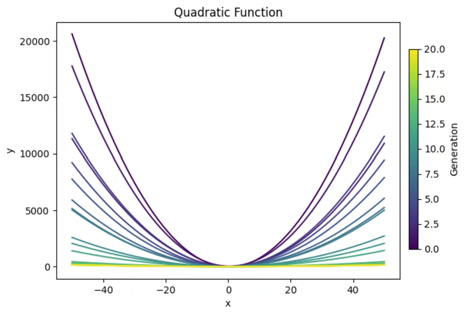
The equation y=ax2+bx+c, when graphed, creates a parabola. We will use a genetic algorithm to find the combination of values for a, b, and c that results in the flattest parabola. Here’s a preview of what we’ll achieve:

Import libraries

At the top of our function, we’ll import the necessary libraries. We’ll be using ‘random’ to generate random values for our starting population. Numpy is generally useful when doing any math, in my opinion. 

And I am a firm believer that you should always make plots to make sure your code is doing what you think it’s doing. So we’ll import ‘matplotlib.pyplot’ to make some graphs.

I also like to print out important results from each generation (assuming a relatively small number of generations) to better understand what happened during the simulation. So we’ll import ‘PrettyTable’ for that.

import random
import matplotlib.pyplot as plt
import numpy as np
from prettytable import PrettyTable

Define fitness function

Next we need to define the fitness function that will evaluate the fitness of every solution. In this case, we want to find the flattest graphed u-shape. So I calculated the y value at the vertex and at x=-1 and x=1. 

Then I calculated the curviness of the graph as the difference in y value at these three points. Since we want to get the flattest curve, I negated curviness to finish off the fitness function.

# Define the fitness function (objective is to create the flattest U-shape)
def fitness_function(params):
    a, b, c = params
    if a <= 0:
        return -float('inf')  # Penalize downward facing u-shapes heavily
    vertex_x = -b / (2 * a) #x value at vertex
    vertex_y = a * (vertex_x ** 2) + b * vertex_x + c #y value at vertex
    y_left = a * (-1) ** 2 + b * (-1) + c #y-coordinate at x = -1
    y_right = a * (1) ** 2 + b * (1) + c #y-coordinate at x = 1
    curviness = abs(y_left - vertex_y) + abs(y_right - vertex_y)
    return -curviness  # Negate to minimize curviness

Create initial population

We will use the ‘random’ library to generate a population of random solutions. Each individual in this population is a set of values for a, b, and c.

# Create the initial population
def create_initial_population(size, lower_bound, upper_bound):
    population = []
    for _ in range(size):
        individual = (random.uniform(lower_bound, upper_bound),
                      random.uniform(lower_bound, upper_bound),
                      random.uniform(lower_bound, upper_bound))
        population.append(individual)
    return population

Create a selection function

The selection function will determine which individuals reproduce to create the next population. In this example, we’ll use a tournament selection process, where a random subset of individuals in the population will be taken, and the individuals with the largest fitness within that subset will be selected for reproduction.

# Selection function using tournament selection
def selection(population, fitnesses, tournament_size=3):
    selected = []
    for _ in range(len(population)):
        tournament = random.sample(list(zip(population, fitnesses)), tournament_size)
        winner = max(tournament, key=lambda x: x[1])[0]
        selected.append(winner)
    return selected

Make a crossover function

Next, we’ll write a quick function to use crossover to create new solutions based on existing solutions.

# Crossover function
def crossover(parent1, parent2):
    alpha = random.random()
    child1 = tuple(alpha * p1 + (1 - alpha) * p2 for p1, p2 in zip(parent1, parent2))
    child2 = tuple(alpha * p2 + (1 - alpha) * p1 for p1, p2 in zip(parent1, parent2))
    return child1, child2

Design a mutation function

We also need a mutation function to introduce randomness to subsequent generations. This is important to make sure there’s enough diversity in each generation to select from.

# Mutation function
def mutation(individual, mutation_rate, lower_bound, upper_bound):
    individual = list(individual)
    for i in range(len(individual)):
        if random.random() < mutation_rate:
            mutation_amount = random.uniform(-1, 1)
            individual[i] += mutation_amount
            # Ensure the individual stays within bounds
            individual[i] = max(min(individual[i], upper_bound), lower_bound)
    return tuple(individual)

Main loop

Next we need to create the main loop that will put all these pieces together to run our algorithm. Since we also need to plot our results, I’ll add in the plotting code in this section, as well as the code needed to create our final table.

# Main genetic algorithm function
def genetic_algorithm(population_size, lower_bound, upper_bound, generations, mutation_rate):
    population = create_initial_population(population_size, lower_bound, upper_bound)
    
    # Prepare for plotting
    fig, axs = plt.subplots(3, 1, figsize=(12, 18))  # 3 rows, 1 column for subplots
    best_performers = []
    all_populations = []

    # Prepare for table
    table = PrettyTable()
    table.field_names = ["Generation", "a", "b", "c", "Fitness"]

    for generation in range(generations):
        fitnesses = [fitness_function(ind) for ind in population]

        # Store the best performer of the current generation
        best_individual = max(population, key=fitness_function)
        best_fitness = fitness_function(best_individual)
        best_performers.append((best_individual, best_fitness))
        all_populations.append(population[:])
        table.add_row([generation + 1, best_individual[0], best_individual[1], best_individual[2], best_fitness])

        population = selection(population, fitnesses)

        next_population = []
        for i in range(0, len(population), 2):
            parent1 = population[i]
            parent2 = population[i + 1]

            child1, child2 = crossover(parent1, parent2)

            next_population.append(mutation(child1, mutation_rate, lower_bound, upper_bound))
            next_population.append(mutation(child2, mutation_rate, lower_bound, upper_bound))

        # Replace the old population with the new one, preserving the best individual
        next_population[0] = best_individual
        population = next_population

    # Print the table
    print(table)

    # Plot the population of one generation (last generation)
    final_population = all_populations[-1]
    final_fitnesses = [fitness_function(ind) for ind in final_population]

    axs[0].scatter(range(len(final_population)), [ind[0] for ind in final_population], color='blue', label='a')
    axs[0].scatter([final_population.index(best_individual)], [best_individual[0]], color='cyan', s=100, label='Best Individual a')
    axs[0].set_ylabel('a', color='blue')
    axs[0].legend(loc='upper left')
    
    axs[1].scatter(range(len(final_population)), [ind[1] for ind in final_population], color='green', label='b')
    axs[1].scatter([final_population.index(best_individual)], [best_individual[1]], color='magenta', s=100, label='Best Individual b')
    axs[1].set_ylabel('b', color='green')
    axs[1].legend(loc='upper left')
    
    axs[2].scatter(range(len(final_population)), [ind[2] for ind in final_population], color='red', label='c')
    axs[2].scatter([final_population.index(best_individual)], [best_individual[2]], color='yellow', s=100, label='Best Individual c')
    axs[2].set_ylabel('c', color='red')
    axs[2].set_xlabel('Individual Index')
    axs[2].legend(loc='upper left')
    
    axs[0].set_title(f'Final Generation ({generations}) Population Solutions')

    # Plot the values of a, b, and c over generations
    generations_list = range(1, len(best_performers) + 1)
    a_values = [ind[0][0] for ind in best_performers]
    b_values = [ind[0][1] for ind in best_performers]
    c_values = [ind[0][2] for ind in best_performers]
    fig, ax = plt.subplots()
    ax.plot(generations_list, a_values, label='a', color='blue')
    ax.plot(generations_list, b_values, label='b', color='green')
    ax.plot(generations_list, c_values, label='c', color='red')
    ax.set_xlabel('Generation')
    ax.set_ylabel('Parameter Values')
    ax.set_title('Parameter Values Over Generations')
    ax.legend()

    # Plot the fitness values over generations
    best_fitness_values = [fit[1] for fit in best_performers]
    min_fitness_values = [min([fitness_function(ind) for ind in population]) for population in all_populations]
    max_fitness_values = [max([fitness_function(ind) for ind in population]) for population in all_populations]
    fig, ax = plt.subplots()
    ax.plot(generations_list, best_fitness_values, label='Best Fitness', color='black')
    ax.fill_between(generations_list, min_fitness_values, max_fitness_values, color='gray', alpha=0.5, label='Fitness Range')
    ax.set_xlabel('Generation')
    ax.set_ylabel('Fitness')
    ax.set_title('Fitness Over Generations')
    ax.legend()

    # Plot the quadratic function for each generation
    fig, ax = plt.subplots()
    colors = plt.cm.viridis(np.linspace(0, 1, generations))
    for i, (best_ind, best_fit) in enumerate(best_performers):
        color = colors[i]
        a, b, c = best_ind
        x_range = np.linspace(lower_bound, upper_bound, 400)
        y_values = a * (x_range ** 2) + b * x_range + c
        ax.plot(x_range, y_values, color=color)

    ax.set_xlabel('x')
    ax.set_ylabel('y')
    ax.set_title('Quadratic Function')

    # Create a subplot for the colorbar
    cax = fig.add_axes([0.92, 0.2, 0.02, 0.6])  # [left, bottom, width, height]
    norm = plt.cm.colors.Normalize(vmin=0, vmax=generations)
    sm = plt.cm.ScalarMappable(cmap='viridis', norm=norm)
    sm.set_array([])
    fig.colorbar(sm, ax=ax, cax=cax, orientation='vertical', label='Generation')

    plt.show()

    return max(population, key=fitness_function)

Making it all run

Lastly, we need to set up the parameters for our algorithm and run it.

# Parameters for the genetic algorithm
population_size = 100
lower_bound = -50
upper_bound = 50
generations = 20
mutation_rate = 1

# Run the genetic algorithm
best_solution = genetic_algorithm(population_size, lower_bound, upper_bound, generations, mutation_rate)
print(f"Best solution found: a = {best_solution[0]}, b = {best_solution[1]}, c = {best_solution[2]}")

Termination condition (optional)

Now in this example, we set a specific number of generations for our algorithm to run. However, we could have alternatively set up a termination condition that stopped the program when we reached a target fitness value. That could look something like this:

def termination_condition(fitnesses, target_fitness):
    return max(fitnesses) >= target_fitness

Putting it all together

Here is the complete code all together.

import random
import matplotlib.pyplot as plt
import numpy as np
from prettytable import PrettyTable

# Define the fitness function (objective is to create the flattest U-shape)
def fitness_function(params):
    a, b, c = params
    if a <= 0:
        return -float('inf')  # Penalize downward facing u-shapes heavily
    vertex_x = -b / (2 * a) #x value at vertex
    vertex_y = a * (vertex_x ** 2) + b * vertex_x + c #y value at vertex
    y_left = a * (-1) ** 2 + b * (-1) + c #y-coordinate at x = -1
    y_right = a * (1) ** 2 + b * (1) + c #y-coordinate at x = 1
    curviness = abs(y_left - vertex_y) + abs(y_right - vertex_y)
    return -curviness  # Negate to minimize curviness

# Create the initial population
def create_initial_population(size, lower_bound, upper_bound):
    population = []
    for _ in range(size):
        individual = (random.uniform(lower_bound, upper_bound),
                      random.uniform(lower_bound, upper_bound),
                      random.uniform(lower_bound, upper_bound))
        population.append(individual)
    return population

# Selection function using tournament selection
def selection(population, fitnesses, tournament_size=3):
    selected = []
    for _ in range(len(population)):
        tournament = random.sample(list(zip(population, fitnesses)), tournament_size)
        winner = max(tournament, key=lambda x: x[1])[0]
        selected.append(winner)
    return selected

# Crossover function
def crossover(parent1, parent2):
    alpha = random.random()
    child1 = tuple(alpha * p1 + (1 - alpha) * p2 for p1, p2 in zip(parent1, parent2))
    child2 = tuple(alpha * p2 + (1 - alpha) * p1 for p1, p2 in zip(parent1, parent2))
    return child1, child2

# Mutation function
def mutation(individual, mutation_rate, lower_bound, upper_bound):
    individual = list(individual)
    for i in range(len(individual)):
        if random.random() < mutation_rate:
            mutation_amount = random.uniform(-1, 1)
            individual[i] += mutation_amount
            # Ensure the individual stays within bounds
            individual[i] = max(min(individual[i], upper_bound), lower_bound)
    return tuple(individual)

# Main genetic algorithm function
def genetic_algorithm(population_size, lower_bound, upper_bound, generations, mutation_rate):
    population = create_initial_population(population_size, lower_bound, upper_bound)
    
    # Prepare for plotting
    fig, axs = plt.subplots(3, 1, figsize=(12, 18))  # 3 rows, 1 column for subplots
    best_performers = []
    all_populations = []

    # Prepare for table
    table = PrettyTable()
    table.field_names = ["Generation", "a", "b", "c", "Fitness"]

    for generation in range(generations):
        fitnesses = [fitness_function(ind) for ind in population]

        # Store the best performer of the current generation
        best_individual = max(population, key=fitness_function)
        best_fitness = fitness_function(best_individual)
        best_performers.append((best_individual, best_fitness))
        all_populations.append(population[:])
        table.add_row([generation + 1, best_individual[0], best_individual[1], best_individual[2], best_fitness])

        population = selection(population, fitnesses)

        next_population = []
        for i in range(0, len(population), 2):
            parent1 = population[i]
            parent2 = population[i + 1]

            child1, child2 = crossover(parent1, parent2)

            next_population.append(mutation(child1, mutation_rate, lower_bound, upper_bound))
            next_population.append(mutation(child2, mutation_rate, lower_bound, upper_bound))

        # Replace the old population with the new one, preserving the best individual
        next_population[0] = best_individual
        population = next_population

    # Print the table
    print(table)

    # Plot the population of one generation (last generation)
    final_population = all_populations[-1]
    final_fitnesses = [fitness_function(ind) for ind in final_population]

    axs[0].scatter(range(len(final_population)), [ind[0] for ind in final_population], color='blue', label='a')
    axs[0].scatter([final_population.index(best_individual)], [best_individual[0]], color='cyan', s=100, label='Best Individual a')
    axs[0].set_ylabel('a', color='blue')
    axs[0].legend(loc='upper left')
    
    axs[1].scatter(range(len(final_population)), [ind[1] for ind in final_population], color='green', label='b')
    axs[1].scatter([final_population.index(best_individual)], [best_individual[1]], color='magenta', s=100, label='Best Individual b')
    axs[1].set_ylabel('b', color='green')
    axs[1].legend(loc='upper left')
    
    axs[2].scatter(range(len(final_population)), [ind[2] for ind in final_population], color='red', label='c')
    axs[2].scatter([final_population.index(best_individual)], [best_individual[2]], color='yellow', s=100, label='Best Individual c')
    axs[2].set_ylabel('c', color='red')
    axs[2].set_xlabel('Individual Index')
    axs[2].legend(loc='upper left')
    
    axs[0].set_title(f'Final Generation ({generations}) Population Solutions')

    # Plot the values of a, b, and c over generations
    generations_list = range(1, len(best_performers) + 1)
    a_values = [ind[0][0] for ind in best_performers]
    b_values = [ind[0][1] for ind in best_performers]
    c_values = [ind[0][2] for ind in best_performers]
    fig, ax = plt.subplots()
    ax.plot(generations_list, a_values, label='a', color='blue')
    ax.plot(generations_list, b_values, label='b', color='green')
    ax.plot(generations_list, c_values, label='c', color='red')
    ax.set_xlabel('Generation')
    ax.set_ylabel('Parameter Values')
    ax.set_title('Parameter Values Over Generations')
    ax.legend()

    # Plot the fitness values over generations
    best_fitness_values = [fit[1] for fit in best_performers]
    min_fitness_values = [min([fitness_function(ind) for ind in population]) for population in all_populations]
    max_fitness_values = [max([fitness_function(ind) for ind in population]) for population in all_populations]
    fig, ax = plt.subplots()
    ax.plot(generations_list, best_fitness_values, label='Best Fitness', color='black')
    ax.fill_between(generations_list, min_fitness_values, max_fitness_values, color='gray', alpha=0.5, label='Fitness Range')
    ax.set_xlabel('Generation')
    ax.set_ylabel('Fitness')
    ax.set_title('Fitness Over Generations')
    ax.legend()

    # Plot the quadratic function for each generation
    fig, ax = plt.subplots()
    colors = plt.cm.viridis(np.linspace(0, 1, generations))
    for i, (best_ind, best_fit) in enumerate(best_performers):
        color = colors[i]
        a, b, c = best_ind
        x_range = np.linspace(lower_bound, upper_bound, 400)
        y_values = a * (x_range ** 2) + b * x_range + c
        ax.plot(x_range, y_values, color=color)

    ax.set_xlabel('x')
    ax.set_ylabel('y')
    ax.set_title('Quadratic Function')

    # Create a subplot for the colorbar
    cax = fig.add_axes([0.92, 0.2, 0.02, 0.6])  # [left, bottom, width, height]
    norm = plt.cm.colors.Normalize(vmin=0, vmax=generations)
    sm = plt.cm.ScalarMappable(cmap='viridis', norm=norm)
    sm.set_array([])
    fig.colorbar(sm, ax=ax, cax=cax, orientation='vertical', label='Generation')

    plt.show()

    return max(population, key=fitness_function)

# Parameters for the genetic algorithm
population_size = 100
lower_bound = -50
upper_bound = 50
generations = 20
mutation_rate = 1

# Run the genetic algorithm
best_solution = genetic_algorithm(population_size, lower_bound, upper_bound, generations, mutation_rate)
print(f"Best solution found: a = {best_solution[0]}, b = {best_solution[1]}, c = {best_solution[2]}")

Evaluating the Results

Let’s use our outputs to see how our function performed.

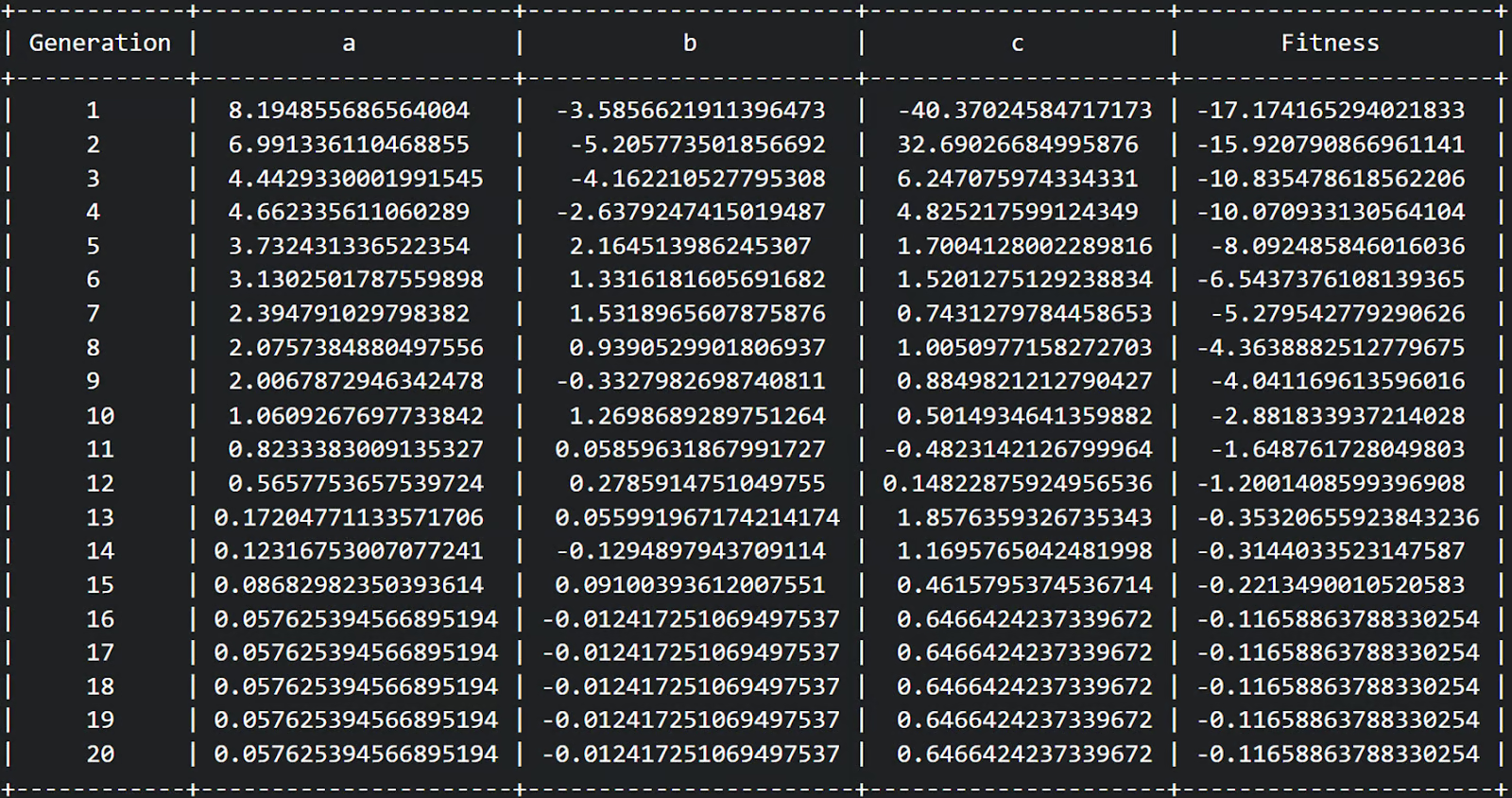
First, we can see from our table that we completed 20 generations and the fitness seemed to increase from a relatively negative fitness to a less negative fitness over each generation. Great!

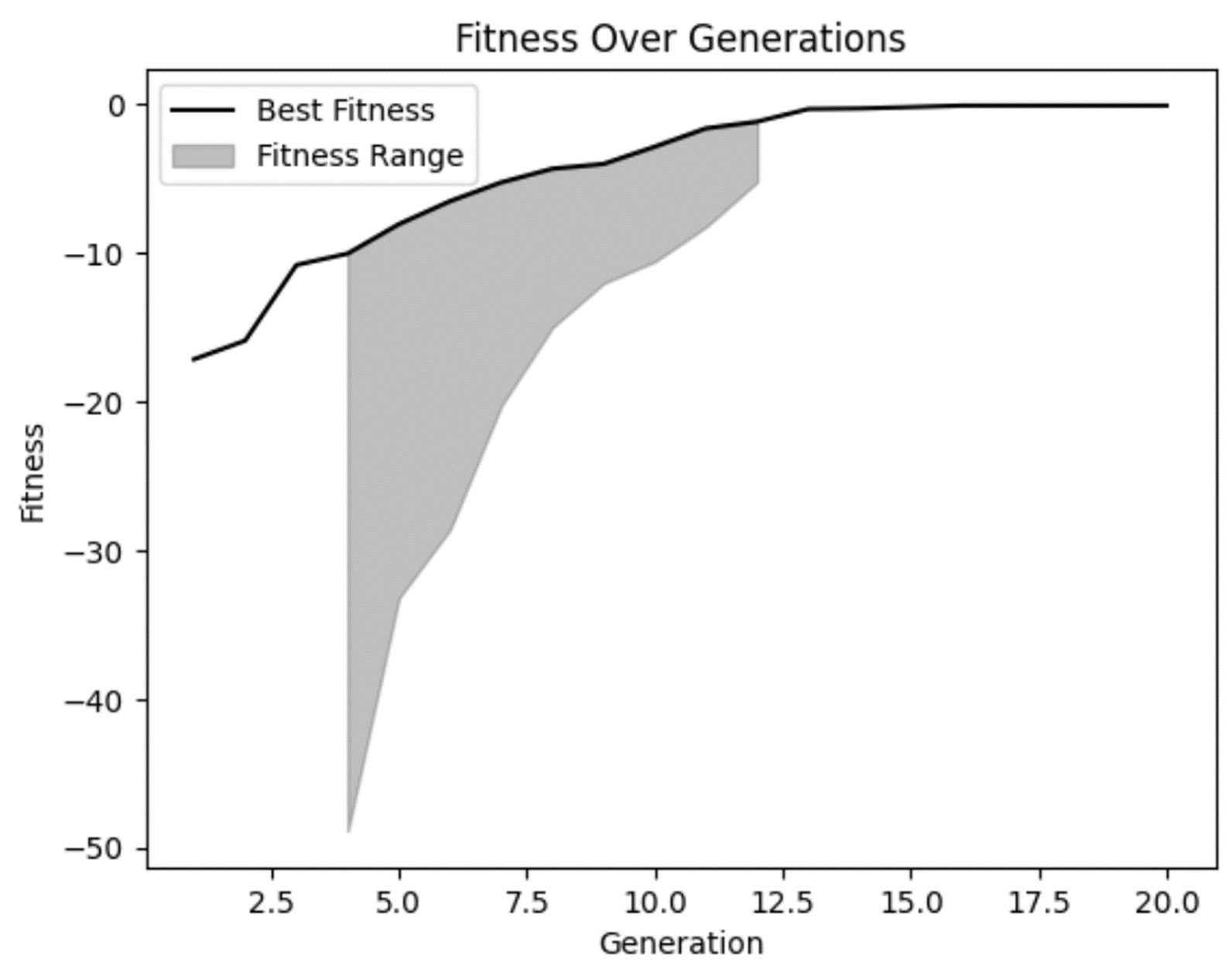
From our fitness graph, we can confirm our suspicions that fitness did improve over time and seems to have flattened out a bit in later generations. But we can also see that in some of the early generations there were some really bad solutions that our model rightly rejected.

We can also see that in several generations there wasn’t a lot of diversity in fitness range. While that isn’t necessarily a bad thing, it is something to watch out for. In some cases, this may be an indicator of premature convergence, which is a problem that occurs when there is not enough diversity in your population.

Next, let’s plot our equations from each generation to see if we really did flatten it out.

We can see that our early generation solutions are very curved, which makes sense. This equation produces a U-shaped graph. But we can also see that future generations became steadily more flat. This is exactly what we were looking for!

Now, it’s worth noting that we are explicitly only looking within our stated bounds of -50 - 50. If we zoomed this graph out, it would show that even these seemingly flat lines are still u-shapes, just with wider bases.

This example highlights the importance of being cautious with our assumptions in analyses to ensure they support our predictions. Our model did exactly what we wanted it to, but only within the bounds we gave it. If we wanted to find a combination of variables that would create a flat shape farther out, then we would need to rerun the model with wider bounds.

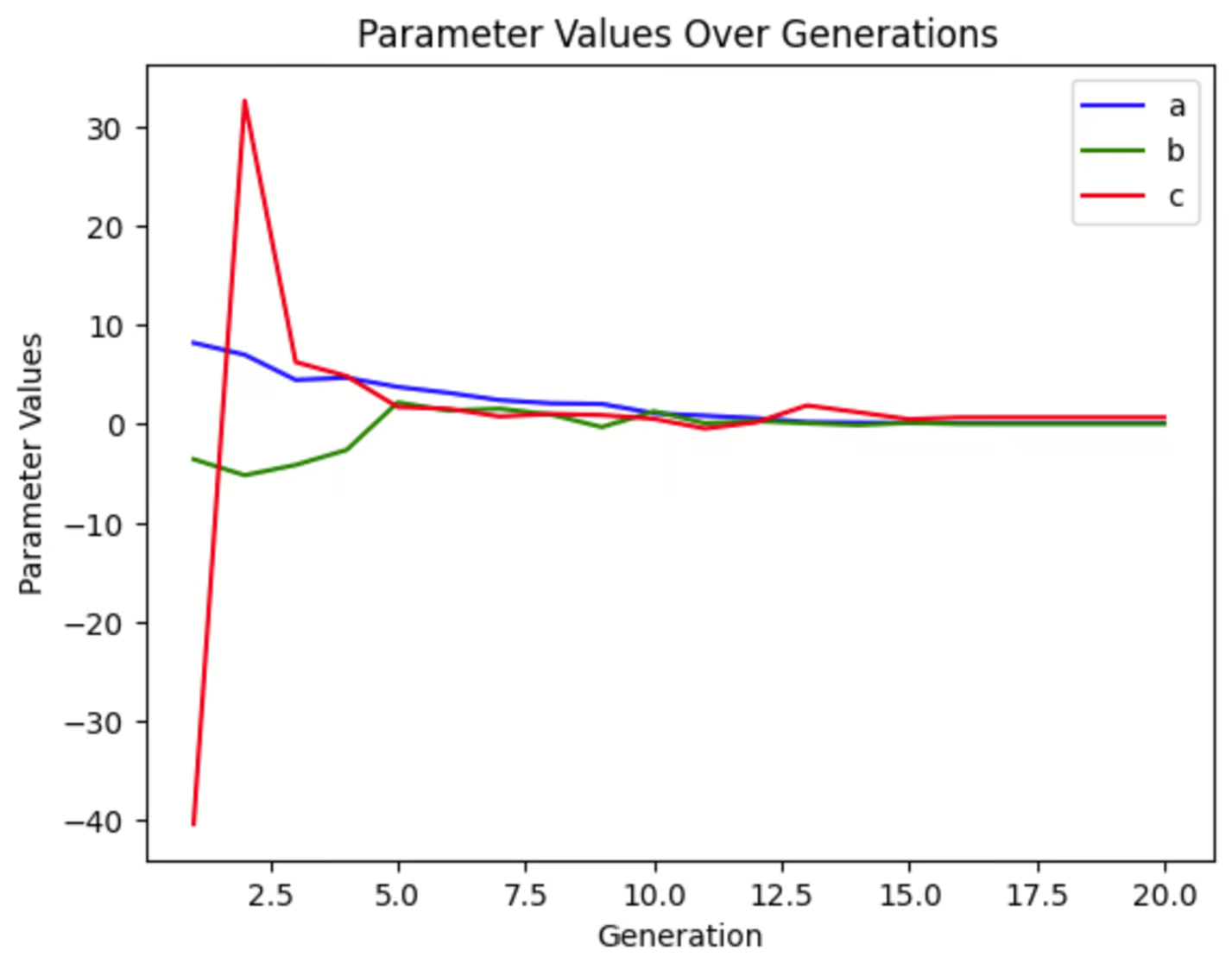
We can plot each of the variables to see how much they changed through the generations. We can see that in this run of the simulation, c varied wildly early on while a and b changed much less dramatically. This graph will look different every time we run this simulation, even if we don’t change any parameters because our starting population is random.

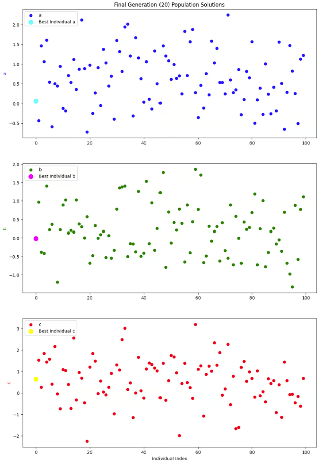
The last graph I want to look at is just a snapshot of the entire population in one generation: the final generation. Since each individual in the population has three parameters, I decided to separate them into three subplots instead of fussing around with 3-dimensional plots. 

What I really want to see from these graphs is whether there is a good diversity within this generation. Without a good amount of diversity, we could end up with a situation where the only solutions available are ones with low fitness values, resulting in premature convergence. But it looks like this graphs shows a good amount of diversity, so I’m happy with this result.

Considerations and Tips

Genetic algorithms can be used in a wide variety of situations. But there are a few considerations to keep in mind.

Parameter tuning

As with any model, the performance of a genetic algorithm depends on various parameters, notably population size, crossover rate, mutation rate, and bounding parameters. Changing these parameters will change how your model performs.

As a general rule of thumb, larger population sizes will help you find the optimal solution quicker because there are more options to choose from. However, larger population sizes also require more time and resources to run.

A higher crossover rate can lead to faster convergence by combining beneficial traits from different individuals more frequently. However, a crossover rate that is too high might disrupt the population structure, leading to premature convergence.

A higher mutation rate helps maintain genetic diversity, preventing the algorithm from getting stuck at a local optimum. However, if the mutation rate is too high, it can disrupt the convergence process by introducing too much randomness, making it difficult for the algorithm to refine solutions.

Bounding parameters define the range within which the algorithm searches for solutions. These are important to tune to your particular business problem. Too narrow of a bounding area may miss optimal solutions to your problem. Too broad of a bounding area will take more time and resources to run. But there are other considerations too. 

For instance, in our coded example above, that equation theoretically has no limits. But practically, we can’t ask the computer to find the flattest arc in an infinitely large graph. So, boundaries are necessary. But changing those boundaries will also change the optimal answer. In my opinion, establishing appropriate boundaries for your specific use case is imperative with any model.

There may be other important parameters to tune in your particular model. Experiment with different values to find the best settings for your problem. To learn about tuning GA’s specifically, check out Informed Methods: Genetic Algorithms.

Encoding

Encoding is an important step in setting up a genetic algorithm. It involves converting potential solutions into a format that the algorithm can process. For example, let’s say we’re designing a genetic algorithm to optimize delivery routes for our trucks. How do you turn a list of delivery locations into a chromosome to put into a GA? Encoding transforms this list into a sequence the algorithm can manipulate, such as an ordered list of locations representing a possible delivery route.

Proper encoding ensures that the genetic algorithm can effectively explore the solution space and combine or mutate solutions in meaningful ways. Without it, the algorithm wouldn't be able to handle complex data. Data like delivery locations, scheduling problems, or customer service interactions are only made accessible to computers through encoding. 

There are several encoding schemas to choose from. You can learn more to decide which might be best for your situation in Working with Categorical Data in Python or How to Convert Strings to Bytes in Python.

Premature convergence

Premature convergence is a problem that occurs when the population becomes too similar. This can result in the algorithm to getting stuck at a local optimum instead of finding the global optimum. Essentially, if there is not enough diversity in the population, the solutions get “inbred” and you don’t get the best solution.

There are a few techniques you can try to avoid premature convergence. A higher mutation rate can introduce more diversity into the population, helping to explore new areas of the solution space. You can also try starting with a more diverse initial population to ensure a wide exploration of the solution space from the beginning.

If you are still dealing with premature convergence, you can try adjusting parameters such as mutation rate and crossover rate dynamically based on the algorithm's progress. Alternatively, you can use multiple populations (think of them as islands) that occasionally exchange individuals to maintain diversity.

You can learn more about premature convergence and other machine learning missteps in the Monitoring Machine Learning Concepts course.

Elitism

On the other hand, strong crossover and mutation or any randomness in selection can mean that great solutions don’t end up reproducing. That’s where elitism can come in. Elitism is a technique where the best individuals are directly carried over to the next generation to preserve good solutions. This helps ensure that the best solutions are not lost during the evolutionary process.

However, be cautious if you use elitism. If elitism is used without a high enough population diversity, you may end up with premature convergence instead. If your business problem calls for elitism techniques, make sure to pair it with strong enough crossover and mutation functions and a large population size. This approach helps maintain a healthy balance between the exploitation of known solutions and the exploration of new possibilities.

Conclusion

Genetic algorithms are a fantastic example of data science drawing inspiration from the natural world. They offer a powerful method for solving complex optimization problems by mimicking the process of natural selection.

If you’re interested in other models inspired by biology, learn about neural networks and other deep learning techniques in Introduction to Deep Learning in Python. You may also be interested in DataCamp’s Generative AI Concepts course and AI Ethics.

If you are inspired to do a project with biological data, check out Analyzing Genomic Data in R or Biomedical Image Analysis in Python.