Welcome to our Excel Basics Cheatsheet! Whether you're new to the program or just need a quick refresher, this guide will help you master the essential skills needed to navigate and utilize the powerful features of Excel efficiently. From working with cells and formulas to flow control and conditional computation, our cheat sheet provides easy-to-follow instructions and examples to help you become a pro at using this popular spreadsheet software. Whether you're a student, professional, or just someone looking to improve your Excel data analysis skills, this cheat sheet is the perfect resource for anyone looking to improve their Excel proficiency.
Explore Excel basics by starting our Excel Fundamentals Track now.
Have this cheat sheet at your fingertips
Download PDFAdvance Your Career with Excel
Gain the skills to maximize Excel—no experience required.
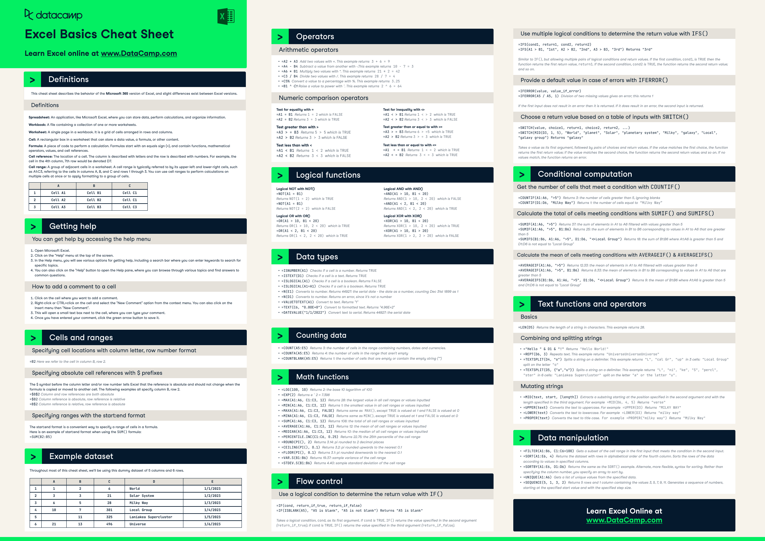
Definitions
This cheat sheet describes the behavior of the Microsoft 365 version of Excel, and slight differences exist between Excel versions.
Spreadsheet: An application, like Microsoft Excel, where you can store data, perform calculations, and organize information.
Workbook: A file containing a collection of one or more worksheets.
Worksheet: A single page in a workbook. It is a grid of cells arranged in rows and columns.
Cell: A rectangular box in a worksheet that can store a data value, a formula, or other content.
Formula: A piece of code to perform a calculation. Formulas start with an equals sign (=), and contain functions, mathematical operators, values, and cell references.
Cell reference: The location of a cell. The column is described with letters and the row is described with numbers. For example, the cell in the 4th column, 7th row would be denoted D7.
Cell range: A group of adjacent cells in a worksheet. A cell range is typically referred to by its upper-left and lower-right cells, such as A1:C3, referring to the cells in columns A, B, and C and rows 1 through 3. You can use cell ranges to perform calculations on multiple cells at once or to apply formatting to a group of cells.
|
A |
B |
C |
|
|
1 |
Cell A1 |
Cell B1 |
Cell C1 |
|
2 |
Cell A2 |
Cell B2 |
Cell C2 |
|
3 |
Cell A3 |
Cell B3 |
Cell C3 |
Getting help
You can get help by accessing the help menu
- Open Microsoft Excel.
- Click on the "Help" menu at the top of the screen.
- In the Help menu, you will see various options for getting help, including a search bar where you can enter keywords to search for specific topics.
- You can also click on the "Help" button to open the Help pane, where you can browse through various topics and find answers to common questions.
How to add a comment to a cell
- Click on the cell where you want to add a comment.
- Right-click or CTRL+click on the cell and select the "New Comment" option from the context menu. You can also click on the Insert menu then "New Comment".
- This will open a small text box next to the cell, where you can type your comment.
- Once you have entered your comment, click the green arrow button to save it.
Cells and ranges
Specifying cell locations with column letter, row number format
=B2 Here we refer to the cell in column B, row 2.
Specifying absolute cell references with $ prefixes
The $ symbol before the column letter and/or row number tells Excel that the reference is absolute and should not change when the formula is copied or moved to another cell. The following examples all specify column B, row 2.
=$B$2 Column and row references are both absolute=$B2 Column reference is absolute, row reference is relative=B$2 Column reference is relative, row reference is absolute
Specifying ranges with the start:end format
The start:end format is a convenient way to specify a range of cells in a formula.
Here is an example of start:end format when using the SUM() formula:=SUM(B2:B5)
Example dataset
Throughout most of this cheat sheet, we’ll be using this dummy dataset of 5 columns and 6 rows.
|
A |
B |
C |
D |
E |
|
|
1 |
1 |
2 |
6 |
World |
1/1/2023 |
|
2 |
3 |
3 |
21 |
Solar System |
1/2/2023 |
|
3 |
6 |
5 |
28 |
Milky Way |
1/3/2023 |
|
4 |
10 |
7 |
301 |
Group |
1/4/2023 |
|
5 |
11 |
325 |
Laniakea Supercluster |
1/5/2023 |
|
|
6 |
21 |
13 |
496 |
Universe |
1/6/2023 |
Operators
Arithmetic operators
=A2 + A3 Add two values with +. This example returns 3 + 6 = 9=A4 - B4 Subtract a value from another with -.This example returns 10 - 7 = 3=A6 * B1 Multiply two values with *. This example returns 21 * 2 = 42=C3 / B4 Divide two values with /. This example returns 28 / 7 = 4=C5% Convert a value to a percentage with %. This example returns 3.25=B1 ^ C1 Raise a value to power with ^. This example returns 2 ^ 6 = 64
Numeric comparison operators
|
Test for equality with =
|
Test for inequality with <>
|
|
Test greater than with >
|
Test greater than or equal to with >=
|
|
Test less than with <
|
Test less than or equal to with <=
|
Logical functions
|
Logical NOT with NOT()
|
Logical AND with AND()
|
|
Logical OR with OR()
|
Logical XOR with XOR()
|
Data types
=ISNUMBER(A1)Checks if a cell is a number. This will return TRUE=ISTEXT(D1)Checks if a cell is a text. This will return TRUE=ISLOGICAL(A1)Checks if a cell is a boolean. This will return FALSE=ISLOGICAL(A1=A1)Checks if a cell is a boolean. This will return TRUE=N(E1)Converts to number. This will return 44927: the serial date - the date as a number, counting Dec 31st 1899 as 1=N(D1)Converts to number. This will return an error, since it’s not a number=VALUETOTEXT(A1)Convert to text. This will return "1"=TEXT(C6, "0.00E+0")Convert to formatted text — This will return "4.96E+2"=DATEVALUE("1/1/2022")Convert text to serial. This will returns 44927: the serial date
Counting data
=COUNT(A5:E5)Returns 3: the number of cells in the range containing numbers, dates and currencies.=COUNTA(A5:E5)Returns 4: the number of cells in the range that aren't empty=COUNTBLANK(A5:E5)Returns 1: the number of cells that are empty or contain the empty string ("")
Math functions
=LOG(100, 10)Returns 2: the base 10 logarithm of 100=EXP(2)Returns e ^ 2 = 7.398=MAX(A1:A6, C1:C3, 12)Returns 28: the largest value in all cell ranges or values inputted=MIN(A1:A6, C1:C3, 12)Returns 1: the smallest value in all cell ranges or values inputted =MAXA(A1:A6, C1:C3, FALSE) Returns same as MAX(), except TRUE is valued at 1 and FALSE is valued at 0=MINA(A1:A6, C1:C3, FALSE)Returns same as MIN(), except TRUE is valued at 1 and FALSE is valued at 0=SUM(A1:A6, C1:C3, 12)Returns 108: the total of all cell ranges or values inputted=AVERAGE(A1:A6, C1:C3, 12)Returns 12: the mean of all cell ranges or values inputted=MEDIAN(A1:A6, C1:C3, 12)Returns 10: the median of all cell ranges or values inputted=PERCENTILE.INC(C1:C6, 0.25)Returns 22.75: the 25th percentile of the cell range=ROUND(PI(), 2)Returns 3.14: pi rounded to 2 decimal places=CEILING(PI(), 0.1)Returns 3.2: pi rounded upwards to the nearest 0.1=FLOOR(PI(), 0.1)Returns 3.1: pi rounded downwards to the nearest 0.1=VAR.S(B1:B6)Returns 19.37: sample variance of the cell range=STDEV.S(B1:B6)Returns 4.40: sample standard deviation of the cell range
Flow control
Use a logical condition to determine the return value with IF(x, yes, no)
=IF(cond, return_if_true, return_if_false)
=IF(ISBLANK(A5), "A5 is blank", "A5 is not blank") Returns "A5 is blank"
Takes a logical condition, cond, as its first argument. If cond is TRUE, IF() returns the value specified in the second argument (return_if_true); if cond is FALSE, IF() returns the value specified in the third argument (return_if_false).
Use a logical condition to determine the return value with IF(x, yes, no)
=IFS(cond1, return1, cond2, return2)
=IFS(A1 > B1, "1st", A2 > B2, "2nd", A3 > B3, "3rd") Returns "3rd"
Similar to IF(), but allowing multiple pairs of logical conditions and return values. If the first condition, cond1, is TRUE then the function returns the first return value, return1. If the second condition is TRUE, the function returns the second return value; and so on.
Provide a default value in case of errors with IFERROR()
=IFERROR(value, value_if_error)
=IFERROR(A5 / A5, 1) Returns 1
If the first input does not result in an error then it is returned. If it does result in an error, the second input is returned.
Choose a return value based on a table of inputs with SWITCH()
=SWITCH(value, choice1, return1, choice2, return2, ...)
=SWITCH(MID(D3, 1, 5), "World", "planet", "Solar", "planetary system", "Milky", "galaxy", "Local", "galaxy group") Returns "galaxy"
Takes a value as its first argument, followed by pairs of choices and return values. If the value matches the first choice, the function returns the first return value; if the value matches the second choice, the function returns the second return value; and so on. If no values match, the function returns an error.
Conditional computation
Get the number of cells that meet a condition with COUNTIF()
=COUNTIF(A1:A6, ">5") Returns 3: the number of cells greater than 5, ignoring blanks
=COUNTIF(D1:D6, "Milky Way") Returns 1: the number of cells equal to “Milky Way”
Calculate the total of cells meeting conditions with SUMIF() and SUMIFS()
=SUMIF(A1:A6, ">5") Returns 37: the sum of elements in A1 to A6 filtered with values greater than 5
=SUMIF(A1:A6, ">5", B1:B6) Returns 25: the sum of elements in B1 to B6 corresponding to values in A1 to A6 that are greater than 5
=SUMIFS(B1:B6, A1:A6, ">5", D1:D6, "<>Local Group") Returns 18: the sum of B1:B6 where A1:A6 is greater than 5 and D1:D6 is not equal to "Local Group"
Calculate the mean of cells meeting conditions with AVERAGEIF() and AVERAGEIFS()
=AVERAGEIF(A1:A6, ">5") Returns 12.33: the mean of elements in A1 to A6 filtered with values greater than 8
=AVERAGEIF(A1:A6, ">5", B1:B6) Returns 8.33: the mean of elements in B1 to B6 corresponding to values in A1 to A6 that are greater than 5
=AVERAGEIFS(B1:B6, A1:A6, ">5", D1:D6, "<>Local Group") Returns 9: the mean of B1:B6 where A1:A6 is greater than 5 and D1:D6 is not equal to "Local Group"
Text functions and operators
Basics
=LEN(D5) Returns the length of a string in characters. This example returns 28.
Combining and splitting strings
="Hello " & D1 & "!"Returns "Hello World!"=REPT(D6, 3)Repeats text. This example returns "UniverseUniverseUniverse"=TEXTSPLIT(D4, "o")Splits a string on a delimiter. This example returns "L", "cal Gr", "up" in 3 cells: "Local Group" split on the letter "o"=TEXTSPLIT(D5, {"a","u"})Splits a string on a delimiter. This example returns "L", "ni", "ke", "S", "percl", "ster" in 6 cells: "Laniakea Supercluster" split on the letter "a" or the letter "u".
Mutating strings
=MID(text, start, [length])Extracts a substring starting at the position specified in the second argument and with the length specified in the third argument. For example =MID(D6, 4, 5) Returns "verse"=UPPER(text)Converts the text to uppercase. For example =UPPER(D3) Returns "MILKY WAY"=LOWER(text)Converts the text to lowercase. For example =LOWER(D3) Returns "milky way"=PROPER(text)Converts the text to title case. For example =PROPER("milky way") Returns "Milky Way"
Data manipulation
=FILTER(A1:B6, C1:C6>100)Gets a subset of the cell range in the first input that meets the condition in the second input.=SORT(A1:E6, 4)Returns the dataset with rows in alphabetical order of the fourth column. Sorts the rows of the data according to values in specified columns.=SORTBY(A1:E6, D1:D6)Returns the same as the SORT() example. Alternate, more flexible, syntax for sorting. Rather than specifying the column number, you specify an array to sort by.=UNIQUE(A1:A6)Gets a list of unique values from the specified data.=SEQUENCE(5, 1, 3, 2)Returns 5 rows and 1 column containing the values 3, 5, 7, 9, 11. Generates a sequence of numbers, starting at the specified start value and with the specified step size
Upskill Your Team in Excel
Excel is just the beginning when it comes to data management and analysis. To truly harness the power of data, your team needs to master a wide range of skills across data science, analytics, and machine learning. DataCamp for Business offers tailored solutions to help organizations upskill their employees, ensuring they are well-equipped to handle the complexities of modern data analytics.
With DataCamp for Business, your team gains access to:
- Vast learning resources: Explore a comprehensive library of interactive courses covering Excel, Python, SQL, Power BI, and more. Custom learning tracks ensure your team focuses on the skills that matter most to your organization.
- Hands-on experience: Build confidence and expertise through active learning, with real-world projects that reinforce key concepts in data ingestion, cleaning, manipulation, visualization, and predictive analytics.
- Scalable solutions: Whether you’re a small startup or a large enterprise, DataCamp provides the tools to upskill, reskill, and foster a data-driven culture, keeping your organization competitive in today’s market.
- Progress tracking: Acess a range of tools to monitor and assess your team’s progress, ensuring they achieve their learning goals.
Investing in DataCamp for Business means empowering your team to make informed, data-driven decisions and tackle complex analytical challenges with confidence. Request a demo today to discover how DataCamp can help your organization thrive.
Master Excel with DataCamp for Business
Equip your team with top-tier Excel skills through DataCamp for Business. Comprehensive training and performance tracking for business success.