How to Use the XLOOKUP Excel Function with Multiple Criteria

XLOOKUP in Excel is currently the newest function of the group of lookup functions (LOOKUP, VLOOKUP, HLOOKUP, and XLOOKUP) that offers many advantages, extended functionality, and greater flexibility.

In this tutorial, we'll first discuss what the XLOOKUP Excel function serves for and how it's better than the older lookup functions; next, we'll take a look at its basic syntax, and then we'll get to the point — the use of the XLOOKUP function with multiple criteria.

If you need to learn the fundamentals of Excel, the beginner-friendly Introduction to Excel course is the right place to start.

Why Use XLOOKUP

The XLOOKUP function searches a range or an array of data and returns the item corresponding to the first match. If no match is found, XLOOKUP can return an approximate match, if a specific match type is provided. In many aspects, the XLOOKUP function surpasses its predecessors in Excel (VLOOKUP, HLOOKUP, and LOOKUP).

In particular, it allows:

• searching for data both horizontally and vertically, and in any direction
• multiple searching criteria
• an approximate match, while defaulting to the exact match
• a partial match
• returning multiple columns and rows
• returning a customized text when no match is found.

In addition, the XLOOKUP function performs faster than the older lookup functions in Excel, which matters when we search within a large amount of data.

XLOOKUP Basic Syntax

Let's briefly overview the basic syntax of the XLOOKUP function:

=XLOOKUP(lookup_value, lookup_array, return_array, [if_not_found], [match_mode], [search_mode]) 

where the required parameters are:

• lookup_value—the value to search for
• lookup_array—the array or range to search
• return_array—the array or range to return

and the optional parameters are:

• [if_not_found]—the supplied text to return where no match is found
• [match_mode]—the match type (exact or approximate), and what to return if no match is found.
• [search_mode]—the search mode to use (direct or reverse search, binary search on the lookup array sorted in ascending or descending order).

We'll see examples of using the optional parameters later in this tutorial.

To learn or brush up on some other helpful functions and formulas in Excel, feel free to check The 15 Basic Excel Formulas Everyone Needs to Know tutorial and Excel Formulas Cheat Sheet.

XLOOKUP with Multiple Criteria

As we see from its basic syntax, the XLOOKUP Excel function is designed to work with a single lookup value of a specified variable by default.

However, we can adapt this function to be used on multiple variables simultaneously, searching for a different lookup value in each variable. In other words, we can conduct our search with XLOOKUP by applying multiple criteria. To do so, there are two main approaches: concatenation and boolean expressions, and we will discuss both of them soon.

Before delving into technical details, let's look at an Excel table we will work with. This table provides information about 10 cats, including their names, colors, and ages:

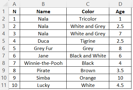
In our experiments, we will use XLOOKUP to find one of the three characteristics of a cat by using the other two.

It's ok that our table is very simple, and we can clearly find what we want in each case without any function. Here, we need to understand the core principles of using XLOOKUP with multiple criteria. Knowing these principles, we can easily extend them to more complex real-world scenarios, e.g., when we have more than two searching criteria or some specific requirements to meet.

XLOOKUP with Multiple Criteria Using Concatenation

The concatenation approach is pretty straightforward: we need to concatenate the corresponding lookup values and arrays between themselves. Let's see how it works.

Suppose we want to find the age of a white-and-grey cat called Nala. For convenience, we added these two criteria on the same sheet where we store our table:

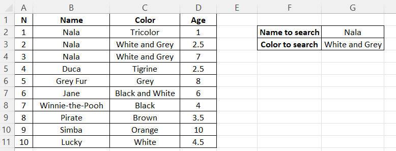
In this case, the formula for XLOOKUP will be as follows:

=XLOOKUP(G2&G3, B2:B11&C2:C11, D2:D11)

It will return 2.5, the age of the first white-and-grey Nala (my cat 😺). Remember that XLOOKUP returns the item corresponding to the first match.

To understand what the first two components of the above formula represent—the ones with an ampersand—we can just run each of them in a separate Excel cell:

=B2:B11&C2:C11

The result is NalaWhite and Grey.

=B2:B11&C2:C11

The result is:

Yes, it's that easy: we just concatenated the corresponding lookup values and lookup arrays between themselves, following the basic XLOOKUP syntax we discussed earlier.

XLOOKUP with Multiple Criteria Using Boolean Expressions

Now, let's perform the same task—finding the age of a white-and-grey cat called Nala—using the second approach: boolean expressions. In this case, the formula for XLOOKUP will be as follows:

=XLOOKUP(1, (B2:B11=G2)*(C2:C11=G3), D2:D11)

As expected, it will also return 2.5, which is the age of the first white-and-grey Nala.

Let's explore the components of the above formula. Here, 1 means TRUE, i.e., we're looking for the TRUE value in the lookup array represented by the second component of the formula—(B2:B11=G2)*(C2:C11=G3).

This component, in turn, contains two multipliers, each checking a certain condition: the first checks if the name corresponds to the name we're looking for, while the second checks if the color corresponds to the color we're looking for. Let's run each multiplier in a separate Excel cell:

=B2:B11=G2

The result is:

=C2:C11=G3

The result is:

Now, let's run the whole second component of the formula:

=(B2:B11=G2)*(C2:C11=G3)

The result is:

While we see two values of 1 in the above result (meaning two TRUE values), the XLOOKUP function returns the item corresponding to the first match.

The approach of using boolean expressions when running the XLOOKUP function for multiple criteria looks much more complicated and less intuitive than the approach based on concatenation. This would become even worse if we used more than two search criteria. Why can't we always use concatenation then?

The boolean expression approach gives us much more flexibility when using XLOOKUP with multiple criteria. Let's take a look at its advantages over the concatenation approach.

Checking the FALSE Value

In the above formula, we were checking if the boolean expression is TRUE, passing in the value of 1:

=XLOOKUP(1, (B2:B11=G2)*(C2:C11=G3), D2:D11)

In some cases, we may need to check if the boolean expression is actually FALSE. For example, we want to find the age of the first cat in our table who is not a white-and-grey Nala. We should modify our formula as follows:

=XLOOKUP(0, (B2:B11=G2)*(C2:C11=G3), D2:D11)

The result will be 1, which is the age of the first cat who is not a white-and-grey Nala (more precisely, it's a tricolor Nala, but not a white-and-grey one).

Using Logical Operators

With boolean expressions, we aren't limited by checking only the equity. Let's say, we want to find the color of a cat called Nala who has less than 2 years:

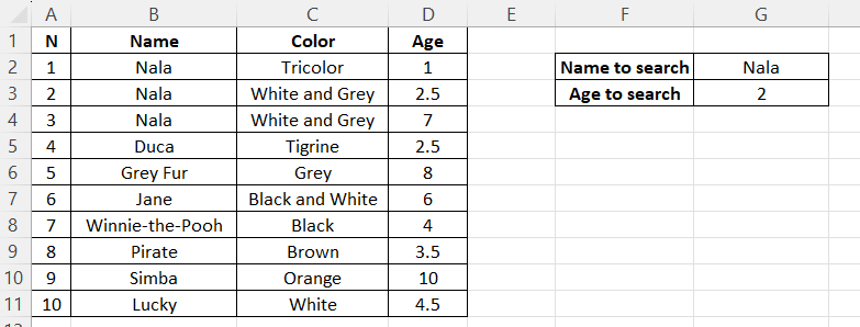
In this case, the formula for XLOOKUP will be as follows:

=XLOOKUP(1, (B2:B11=G2)*(D2:D11<G3), C2:C11)

The result will be Tricolor.

Meeting At Least One Criterion

What we were doing so far was checking the correspondence to all provided criteria. In other scenarios, we may need to meet at least one criterion.

To see how it works, let's return to our initial task—finding the age of a white-and-grey cat called Nala:

This time, however, we want to find the age of a cat who is either called Nala or white-and-grey. The XLOOKUP formula in this case will be:

=XLOOKUP(1, (B2:B11=G2)+(C2:C11=G3), D2:D11)

It returns 1, which is the age of a tricolor Nala.

As a reminder, when we were searching for the age of a cat who is both called Nala and white-and-grey, the formula was as follows:

=XLOOKUP(1, (B2:B11=G2)*(C2:C11=G3), D2:D11)

Substituting * with + made the difference.

If you're interested in discovering Excel’s full potential, consider a comprehensive, practice-oriented, and well-rounded Excel Fundamentals skill path.

Optional Parameters for XLOOKUP with Multiple Criteria

Like a regular usage of XLOOKUP with a single criterion, we can use additional options of this function when running it on multiple criteria. This is where the optional parameters [if_not_found], [match_mode], and [search_mode] come into play.

Let's take a quick look at the examples of using each of these parameters with XLOOKUP and multiple criteria. For simplicity, we'll apply the concatenation approach in each example.

Returning a Supplied Text When No Match Is Found

Here we're searching for the age of a black Nala—an inexistent cat in our table:

In this case, we added to the XLOOKUP formula the optional parameter [if_not_found], to which we assigned the text to be returned if no match is found:

=XLOOKUP(G2&G3, B2:B11&C2:C11, D2:D11, "No cat is found")

Indeed, the function returned the provided text: No cat is found. If we didn't provide any text, the function would have returned #N/A.

Returning an Approximate Match

Let's say, we're looking for the age of a tricolor Nala, but we aren't sure if her color is written as "Tricolor" or "Tricolour" in the table. This is where we need to use an approximate wildcard-based match and pass to the XLOOKUP function the [match_mode] argument equal to 2.

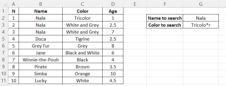
In the above table, we used an asterisk (*), representing any number of characters, including 0. Other wildcards can be found in the Microsoft Office documentation.

The XLOOKUP formula here will be:

=XLOOKUP(G2&G3, B2:B11&C2:C11, D2:D11, , 2)

And it will return 1, the age of the first (and the only) tricolor Nala in our table.

Note that argument 2 in the above formula means that we're interested in an approximate match, rather than searching for the age of a cat Nala of the color "Tricolo*r." In our case, the asterisk captured the word "Tricolor," but it would do the same job on the words "Tricolour" or, say, "Tricolooor."

Performing a Reverse Search

Let's do the same exercise as in the beginning—finding the age of a white-and-grey Nala—but this time, we'll start our search from the last item.

To do so, we need to add to the XLOOKUP function the optional parameter [search_mode] set to -1, as below:

=XLOOKUP(G2&G3, B2:B11&C2:C11, D2:D11, , , -1)

The function returns 7, the age of the first white-and-grey Nala from the end of the lookup array.

Old Approach to Multiple Criteria Search: INDEX and MATCH

In older versions of Excel, to reproduce functionality similar to using the XLOOKUP function with multiple criteria, we need to combine the INDEX and MATCH functions. Without diving into the syntax of both functions, let's see how we can find the age of the first white-and-grey Nala by using the old method INDEX + MATCH and the new XLOOKUP function (for the cell references, we can consult the previous table):

=INDEX(D2:D11, MATCH(1, (G2=B2:B11)*(G3=C2:C11), 0))
=XLOOKUP(1, (B2:B11=G2)*(C2:C11=G3), D2:D11)

While the arguments look somewhat similar, let's mention the main advantages of running the XLOOKUP function over the old method:

• One function is enough for this operation — combining functions is unnecessary.
• The possibility of applying the concatenation approach when possible.
• The possibility of using the optional parameters (the MATCH function lacks them).