Big O Notation and Time Complexity Guide: Intuition and Math

Time complexity analysis provides a way to analyze and predict the efficiency of algorithms in a way that is independent of both the language in which we implement them and the hardware in which they’re executed.

The goal of time complexity analysis isn’t to predict the exact runtime of an algorithm but rather to be able to answer these questions:

1. Given two algorithms that solve the same problem, which one is expected to run faster if the same amount of data is provided to both?
2. If we doubled the data provided to the algorithm, how would the execution time be affected? Will it scale linearly and double as well? Will it remain the same? Or something else entirely?

By the end of this article, you’ll know how to analyze the time complexity of an algorithm and answer these questions.

Does Time Complexity Still Matter in 2024?

Computers are getting faster and faster so one might wonder if there’s any need anymore in worrying about time complexity. Surely nowadays a supercomputer can handle any problem regardless of the algorithm we use to solve it, right?

Well, not quite. The AI boom is largely due to immense advances in hardware performance in recent years.  However, even on the most advanced hardware, simple problems can lead to catastrophic performance if a slow algorithm is used.

For example, imagine using a naive algorithm to sort a database table with ten million entries. Even on a modern computer, this simple operation would take several days to complete, making the database unusable for any practice application. By contrast, using an efficient algorithm, we can expect it to take less than one-tenth of a second.

Basic Operations and Basic Instructions

We analyze an algorithm using the Random Access Machine (RAM or RA-machine) model. This model assumes the following operations take exactly one time step:

• Arithmetic operations
• Logic operations (<, >, ==, etc.)
• Statements like if or return
• Accessing a memory location, such as writing or reading a variable value

These operations are called basic operations. A line of code that executes a constant number of basic operations is called a basic instruction.

Because the number of operations in a basic instruction is constant, it doesn’t depend on the amount of data. Since we care about how the execution time grows as the amount of data grows, we can focus on counting the number of basic instructions the algorithm performs.

Function calls and loops like for and while are evaluated by adding up the number of basic instructions inside of them. Consider the following code that sums the elements of a list.

def sum_list(lst):
  total = 0          # 1 instruction
  for value in lst:    
    total += value   # executed len(lst) times
  return total       # 1 instruction

We added comments to each line to help visualize the number of basic instructions. If N is the length of lst, then the total number of basic instructions is 1 + N + 1 = N + 2.

Big-O Notation

Imagine we have two sorting algorithms. We calculated the number of basic instructions for each of them and got the following expressions:

At first glance, it’s not obvious which one scales better. Big-O notation gives a way to simplify these expressions further by applying these simplifications:

1. Drop the terms with lower exponents
2. Remove multiplicative constants

If we apply this process to both expressions, we get N2 in both cases:

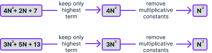
The expression we obtain after simplifying is the algorithm's time complexity, which we denote using O(). In this case, we can write that 4N2 + 2N + 7 = O(N2) and 3N2 + 5N + 13 = O(N2). This means that both algorithms have the same time complexity, which is proportional to the square of the list's number of elements.

Above, we calculated that the sum_list algorithm performed N + 2 operations, where N is the length of the list. Applying the same simplifications, we obtain N, so the time complexity of sum_list is O(N).

This means that the execution time is proportional to the list size. This is expected because when computing the sum, doubling the number of elements in a list should require double the amount of work, not less, not more.

Big-O notation: intuitive explanation

We can ignore the lower terms because, as N grows, their impact on the total sum becomes insignificant when compared to the highest term. The following plot shows the contribution of each of the three terms 4N2, 2N, and 7 to the total sum.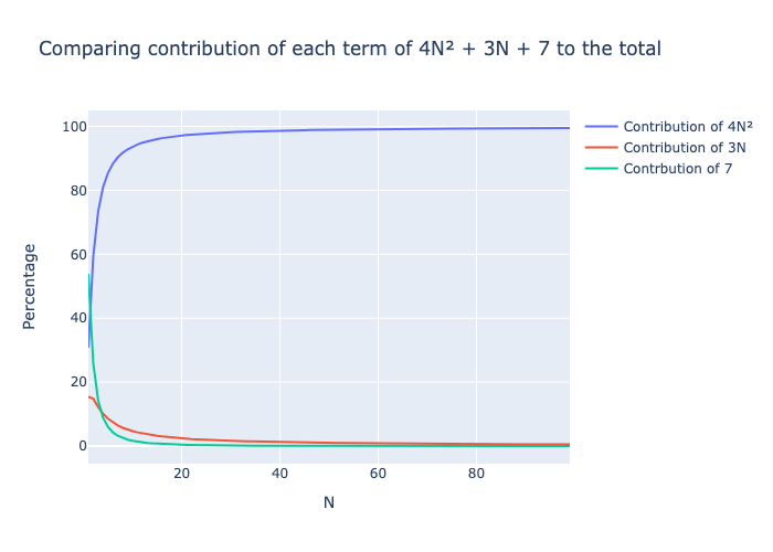

The quadratic term 4N2 very quickly accounts for almost 100% of the total number of operations even for small values of N. Therefore, when dealing with large amounts of data, the time corresponding to lower-order terms will be negligible compared to the higher-order terms. 

We drop the multiplicative constant because this value is independent of the amount of data.

Big-O notation: mathematical definition

The above steps are sufficient for most practical purposes to accurately derive an algorithm’s time complexity. We can count the number of basic instructions an algorithm performs and obtain some expression f(N). After applying the two simplification steps, we obtain some simplified expression g(N). Then, we can write that f(N) = O(g(N)). We read it as “f is big O of g.”

However, this isn’t a formal mathematical definition, and in some cases, it isn’t sufficient. 

The mathematical definition is that a positive function f(N) = O(g(N)) if we can find a constant C such that for large values of N, the following holds:

f(N) ≤ C × g(N)

We can use the definition to show that f(N) = 4N2 + 2N + 7 = O(N2). In this case, we can choose C = 5 and see that for any N > 4,  f(N) ≤ 5 × N2:

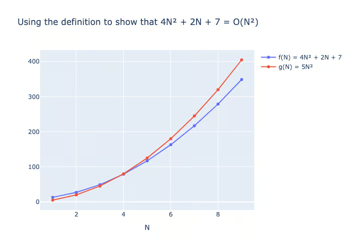
In practice, we’ll just use the above simplification rules.

Types of Time Complexity

Now that we understand the basics of Big-O notation, let's explore common time complexities and their implications, starting with the most efficient: constant time.

Constant time: O(1)

As the name suggests, constant-time algorithms have a constant time complexity, meaning their performance does not depend on the amount of data. These algorithms typically involve calculations with a fixed number of inputs, such as computing the distance between two points.

The distance between two points is calculated by computing the square root of the difference between the x and y coordinates of the two points.

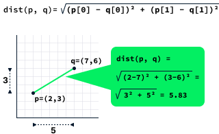
The dist function shown below computes the distance between two points. It consists of three basic instructions, which is a constant. In this case, we write that the time complexity is O(1).

def dist(p, q):
  dx = (p[0] - q[0]) ** 2  # 1 instruction
  dy = (p[1] - q[1]) ** 2  # 1 instruction
  return (dx + dy) ** 0.5  # 1 instruction

Interestingly, it is entirely possible for a function to exhibit constant time complexity, even when processing large datasets. Take, for instance, the case of calculating the length of a list using the len function. This operation is O(1) because the implementation internally keeps track of the list's size, eliminating the need to count the elements each time the length is requested.

Linear time: O(N)

We have previously discussed sum_list as a linear time function example. Generally, linear time algorithms execute tasks that need to inspect each data point individually. Calculating the minimum, maximum, or average is a typical operation in this category.

Let’s practice by analyzing the following function for computing the minimum value of a list:

def minimum(lst):
  min_value = lst[0]                    # 1 instruction
  for i in range(1, len(lst)):
    min_value = min(min_value, lst[i])  # executed len(lst) - 1 times
  return min_value                      # 1 instruction

If the list has N elements, the complexity is 1 + (N - 1) + 1 = N + 1 = O(N).

The execution time of linear time algorithms is directly proportional to the amount of data. Thus, if the amount of data is doubled, the time it takes for the algorithm to process the data should also doubled.

Logarithmic time: O(log(N))

The number-guessing game involves attempting to guess a hidden number between 1 and N, aiming to identify this number with the fewest possible guesses. After every guess, we receive feedback indicating whether the hidden number is higher, lower, or the same as their guess. If the guess is correct, we win the game; otherwise, we continue guessing.

One effective strategy for this game is to consistently guess the midpoint. Suppose N = 15. In this case, our first guess would be 8. If the secret number is smaller than 8, we know it must be between 1 and 7. If it's larger, then it lies between 9 and 15. We continue to guess the midpoint of the remaining range until we find the correct answer. The diagram below illustrates the potential paths this strategy can follow.

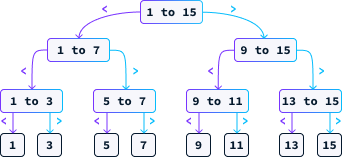
Let's examine the time complexity of this approach. Unlike the previous examples, the number of steps this algorithm takes isn't solely dependent on the input size N, as there's a possibility of guessing correctly on the first attempt.

When analyzing these algorithms, we concentrate on the worst-case scenario. For instance, with N = 15, in the worst case, we would need to make 4 guesses. Each guess, being the midpoint, eliminates half of the remaining possibilities. In the worst-case scenario, we continue guessing until only one possibility remains. Therefore, the question we need to address is:

How many times must we divide N by 2 to obtain 1?

The answer is the base-2 logarithm of N, denoted as log2(N). The algorithm deployed to pinpoint the correct number is known as binary search. Given that the maximum number of guesses is log2(N), we can express its complexity as O(log2(N)) or simply O(log(N)) since constants are insignificant in time complexity notation.

Due to its extremely slow growth rate, logarithmic time complexity is highly sought after in practice, behaving almost like constant time complexity. Even for large values of N, the total number of operations remains remarkably low. For instance, even if N is one billion, the number of operations required is only about 30.

Binary search is a fundamental algorithm in computer science with numerous applications. For example, in natural language processing, spell checkers and autocorrect systems can utilize binary search variants to efficiently identify potential candidate words.

Quadratic time: O(N2)

Sorting data is a fundamental task that computers frequently need to perform. One method to sort a list of N numbers involves iteratively identifying the minimum element of the list.

def selection_sort(lst):
  sorted_lst = []              # 1 instruction
  for _ in range(len(lst)):
    minimum = min(lst)         # executed len(lst) times
    lst.remove(minimum)        # executed len(lst) times
    sorted_lst.append(minimum) # executed len(lst) times
  return sorted_lst            # 1 instruction

To analyze the complexity of a for loop, we evaluate the complexity of the instructions within it and then multiply that result by the number of iterations the loop is executed.

Computing the minimum of a list and removing an element from a list are both O(N) operations. Appending is done in constant time, O(1). Therefore, each iteration of the for loop has a complexity of O(N + N + 1) = O(2N + 1), which simplifies to O(N). Since there are N iterations, the complexity is N × O(N) = O(N2). The rest of the selection_sort() function consists of three simple instructions, so the overall complexity is O(N2 + 3) = O(N2).

Our analysis of the for loop involved an oversimplification. In each iteration, we remove one element from the list, meaning not all iterations execute the same number of instructions. The first iteration executes N instructions, the second executes N - 1, the third N - 2, and this pattern continues until the last iteration, which only executes 1 instruction.

This implies that the true complexity of the for loop is:

N + (N - 1) + (N - 2) + … + 1 

This sum can be shown to be equal to (N2 + N) / 2. However,

(N2 + N) / 2 = ½N2 + ½N = O(N2)

Even though we overcounted, the overall complexity is still quadratic. The selection_sort() function exemplifies a slower sorting algorithm due to its quadratic complexity, O(N2). 

Functions with quadratic complexity scale poorly, making them suitable for small lists but impractical for sorting millions of data points, as they can take days to complete the task. Doubling the amount of data leads to a quadrupling of the execution time.

Loglinear time: O(N log(N))

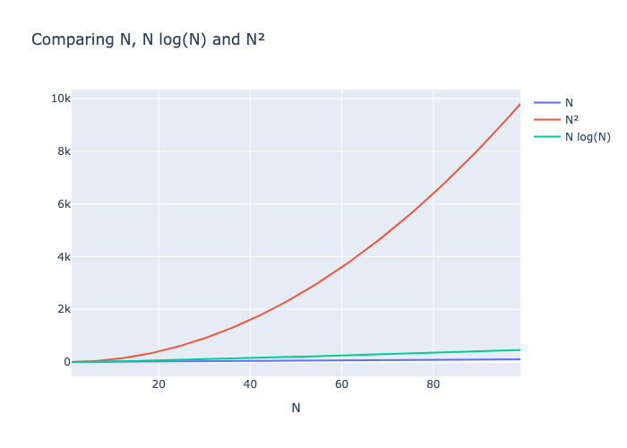
It is possible to devise an algorithm for sorting a list with O(N log(N)) time complexity. One such algorithm is called merge sort.  We won’t go into the details of its implementation, but if you want to learn more about it, check out this quick introduction to merge sort from this course on Data Structures and Algorithms in Python.

As mentioned previously, logarithmic complexity behaves similarly to constant complexity in practice. Therefore, the execution time of an O(N log(N)) algorithm can be comparable to that of a linear-time algorithm in real-world applications.

The following plot shows that N log(N) and N grow at similar rates while N2 grows very fast, quickly becoming very slow.

Cubic time: O(N3)

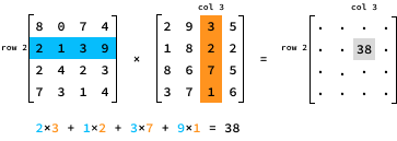
A widely used cubic time complexity algorithm in AI is matrix multiplication, which plays a crucial role in the functionality of large language models like GPT. This algorithm is pivotal to the calculations carried out during both the training and inference phases.

To multiply two N by N matrices, A and B, we need to multiply each row of the first matrix A by each column of the second matrix B. Specifically, the value of the product at entry (i, j) is determined by multiplying the elements in row i of A by the corresponding elements in column j of B.

Here’s a Python implementation of matrix multiplication:

def matrix_mul(A, B):
  n = len(A)                                       # 1 instruction
  res = [[0 for _ in range(n)] for _ in range(n)]  # N^2 instructions
  for i in range(n):
    for j in range(n):
      for k in range(n):
        res[i][j] += A[i][k] * B[k][j]             # executed N×N×N = N^3 times
  return res                                       # 1 instruction

In total,  matrix_mul() executes N3 + N2 + 2 instructions so its time complexity is O(N3).

Alternatively, we could have analyzed the complexity by reasoning about the calculations. The result of the matrix multiplication has N2 entries. Each entry takes O(N) time to compute, so the overall complexity is N2 × O(N) = O(N3).

Cubic time algorithms are quite slow. Doubling the amount of data results in a factor of eight in the execution time, making such algorithms scale very poorly. Even for a relatively small value of N, the number of instructions explodes very quickly.

Matrix multiplication is an example of a computational challenge where advances in hardware have made a significant impact. Although there are slightly more efficient algorithms for matrix multiplication, it is primarily the advances in the design of GPU chips — tailored specifically for performing matrix multiplication — that have significantly facilitated the training of large models like GPT within reasonable timeframes.

More recently, researchers have proposed eliminating matrix multiplication from large learning models—you can read more about this in this article on MatMul-Free LLMs: Key Concepts Explained.

Exponential time complexity: O(2N) and O(N!)

Exponential time algorithms typically arise when a problem is solved by exploring all possible solutions. Consider planning a route for a delivery truck required to visit N delivery locations. One approach to address this problem is to evaluate every possible delivery order. The Python itertools package offers a straightforward method to cycle through all permutations of a list.

import itertools
for order in itertools.permutations([1, 2, 3]):
  print(order)

(1, 2, 3)
(1, 3, 2)
(2, 1, 3)
(2, 3, 1)
(3, 1, 2)
(3, 2, 1)

The number of permutations of a list of length N is denoted by N!, read as "N factorial." The factorial function exhibits exponential growth. For instance, when N = 13, the number of permutations exceeds 1 billion.

Suppose the delivery locations are given as a list of 2D points. In that case, we can determine the delivery sequence that minimizes the total distance by iterating through all possible sequences while keeping track of the best one.

def optimize_route(locations):
  minimum_distance = float("inf")                  # 1 instruction
  best_order = None                                # 1 instruction
  for order in itertools.permutations(locations):  # N! iterations
    distance = 0                                   # 1 instruction, N! times
    for i in range(1, len(order)):                 
      distance += dist(order[i - 1], order[i])     # N-1 instructions, N! times
    if distance < minimum_distance:                
      distance = minimum_distance                  # 1 instruction, N! times
      best_order = order                           # 1 instruction, N! times
  return best_order                                # 1 instruction

The first for loop is executed N! times. Therefore, the number of operations in optimize_route() is N! x (1 + N - 1 + 2) + 3 = N! x (N + 2) + 3 = N! x N + 2N! + 3.

We learned that when calculating time complexity, we ignore lower exponent terms. However, in this scenario, we encounter an N! term, which isn’t a power of N. We can refine our simplification strategy by choosing to omit the terms with slower growth rates. The table below lists terms commonly found in an algorithm's time complexity, arranged from lowest to highest growth rate.

Thus, we can express the time complexity of optimize_route() as N! x N + 2N! + 3 = O(N! x N).

Exponential time complexity algorithms are typically only efficient for solving very small instances. Even with just 13 locations, the number of permutations exceeds 1 billion, rendering this algorithm impractical for real-world scenarios.

Time Complexity: Worst Case and Best Case

With the number-guessing game, we focused on the worst-case complexity. By focusing on the worst case, we guarantee the rate of growth of the algorithm's execution time.

In the best case, we guess the first time, so a best-case complexity analysis would result in O(1) complexity. This is accurate—in the best case, we need a single constant operation. However, this isn’t quite useful because it is very unlikely.

In general, when we analyze the complexity of an algorithm, we always focus on the worst case because:

1. Guarantee of performance: By focusing on the worst-case complexity, we can ensure that our algorithm will never perform worse than a certain threshold. This is crucial for applications that require reliable performance, such as real-time systems, where delays can cause significant issues.
2. Safety and reliability: Worst-case analysis helps design robust algorithms that can handle the most demanding scenarios. It ensures that the algorithm will still function within acceptable limits even in the worst possible situations.
3. Upper bound: Knowing the worst-case complexity gives us an upper bound on the performance. This is useful for understanding the maximum resources (time, memory) an algorithm might require.

Time Complexity: Practical Implications

Time complexity may seem like a very theoretical subject, but it can prove very useful in practice.

For example, if a function consistently handles a small dataset, an easy-to-understand O(N2) algorithm may be more appropriate than a complex and difficult-to-maintain O(N) algorithm. However, this should be a deliberate decision to avoid being caught off-guard when the application cannot handle increased user traffic.

Time complexity analysis reveals that minor code optimizations have a negligible effect on an algorithm's execution time. Significant improvements are achieved by fundamentally reducing the number of basic operations needed to compute the result. Generally, maintaining clean and comprehensible code is preferable over optimizing it to the extent that it becomes unintelligible.

Slower parts of the code will dominate the others. It’s usually pointless to optimize the faster part before optimizing the slower one. For example, imagine we have a function that performs two tasks:

def process_data(data):
  clean_data(data)
  analyze_data(data)

If the clean_data() function has complexity O(N2) and analyze_data() has complexity O(N3), then reducing the complexity of clean_data() will not improve the overall complexity of process_data(). It’s better to focus on improving the analyze_data() function.

Furthermore, time complexity can inform hardware decisions. For example, an O(N3) algorithm, despite its poor scalability, might still be fast enough for tasks with limited data if run on superior hardware or a faster programming language. Conversely, if an algorithm has an exponential time complexity O(2N), no hardware upgrade will suffice, indicating the necessity for a more efficient algorithm.

Conclusion

Despite computers getting faster, we're dealing with more data than ever. Think of it like this: every time we use the Internet, smartphones, or smart home devices, we create tons of information. As this mountain of data grows, sorting through it and finding what's important becomes harder. That's why it's really important to keep making our tools—especially algorithms—better at handling and understanding all this information.

Time complexity analysis offers a straightforward framework for reasoning about an algorithm's execution time. Its primary goal is to provide insights into the growth rate of the time complexity rather than predicting exact execution times. Despite the model's numerous simplifications and assumptions, it has proven to be extremely useful in practice, effectively capturing the essence of algorithm execution time behaviors.

If you want to explore more computer science subjects, check out my article on Data Structures: A Comprehensive Guide With Python Examples.