JEPA Architecture Explained: How LeCun's World Model Works

Imagine you are watching a video of someone throwing a ball across a park, and you pause it halfway. You can guess where the ball will land, but can you guess how every leaf on the trees behind it will move, or how the clouds will move in the next second? Probably not, but the question is, do we really care about those details?

This is the whole point of the Joint Embedding Predictive Architecture, or JEPA for short. 

Most AI models we use today learn by predicting the exact next thing, such as a large language model (LLM) predicting the next token and an image generator predicting every next pixel. 

JEPA, however, predicts a short summary of what comes next, so it can focus on the ball and ignore the leaves.

In very simple language, JEPA teaches an AI to guess the meaning of what is missing instead of redrawing it.

In this article, we will explore what JEPA is, how its three parts work, the full model family from I-JEPA to V-JEPA 2.1, and where it fits next to LLMs in 2026.

Before we start, I would recommend reading about neural networks if you are not confident in them.

What Is JEPA?

Let’s start off by formally defining JEPA:

A Joint Embedding Predictive Architecture (JEPA) is a self-supervised learning approach where a model sees part of some data, turns it into an embedding, and then predicts the embedding of the missing part, instead of predicting the missing pixels or words themselves.

An embedding is just a list of numbers that summarizes something (I like to think of it as a fingerprint). Two photos of the same dog in slightly different light should have very similar embeddings, even though thousands of their pixels are different.

JEPA was proposed by Yann LeCun in his position paper A Path Towards Autonomous Machine Intelligence in 2022, while he was Chief AI Scientist at Meta. 

The paper was less about one specific model and more of a blueprint for building machines that learn the way children and animals do (we will come back to this blueprint later on).

Why the word “predictive” matters

In my opinion, the most important word in the name is “predictive”. 

Older methods such as CLIP and SimCLR also work with embeddings, but they only check whether two embeddings match. 

JEPA goes a step further and asks the model to predict one embedding from another, which is very close to how a world model predicts the next state of its environment.

Imagine a friend telling you about a film you have not seen yet. They will not replay every frame to you, but rather, just tell you what happens, and this summary is all you would need to guess what the sequel might be about.

JEPA vs. generative and contrastive models

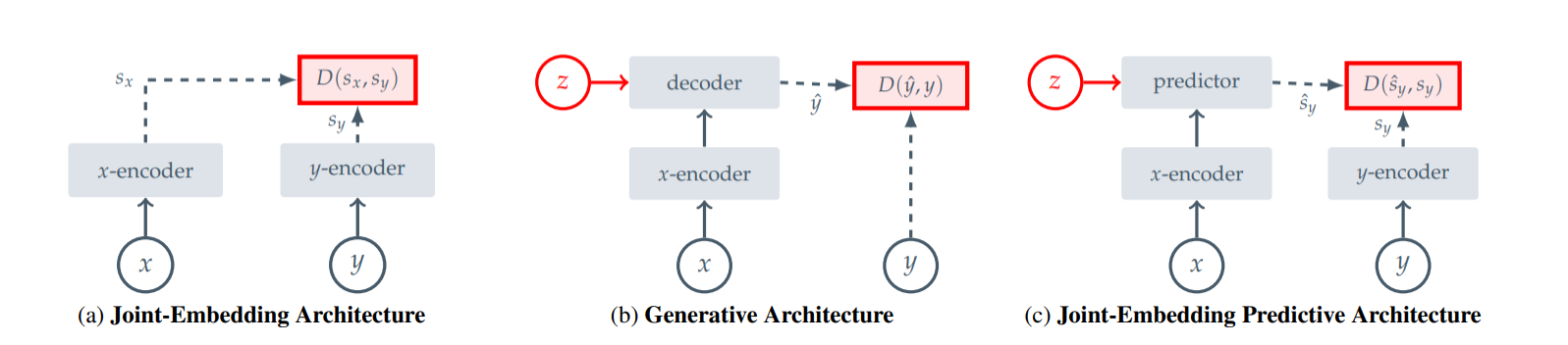
Source: Assran et al., 2023, Self-Supervised Learning from Images with a Joint-Embedding Predictive Architecture, Figure 2.

I have created a table comparing JEPA with the two other big families of self-supervised learning. 

Don’t worry if some of the model names are new; the rows are what matter here:

The row I would focus on is the fourth one. 

A generative model gets penalized for getting the color of every leaf wrong, so it wastes effort on details we don’t really care about. 

JEPA, however, only gets penalized if its summary is wrong, so it is free to ignore the leaves and focus on the ball.

JEPA vs. large language models

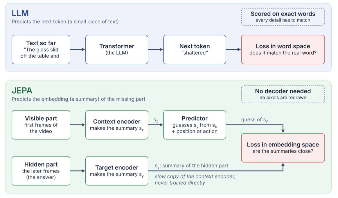
Image by Author

Now let’s compare JEPA with the model we use every day. 

As I said before, an LLM predicts the next token, which is a small piece of text, such as a word or part of a word. JEPA predicts the embedding of a future (or hidden) state, which describes the situation without spelling out every detail.

Let me give you another example of a glass on the edge of the table. 

Give an LLM the sentence “The glass slid off the table and” and it will predict the word “shattered”, because that word appears after similar sentences in its training text. 

However, if you give V-JEPA 2 the first few frames of a video of that glass, it predicts an embedding of the later frames, which captures something like “glass on the floor, in pieces” without drawing where every shard landed.

Both answers do sound sensible, but they come from very different places:

• The LLM’s answer comes from reading text written by people who have seen glasses break.
• V-JEPA 2’s answer comes from watching over 1 million hours of video of things falling, rolling, and colliding.
• Only the second kind of prediction can be linked to a robot’s action (which is exactly what V-JEPA 2-AC adds), so the robot can check what happens if it moves its arm 5 cm to the left.

In short, LLMs predict what will be written next (the next token), while JEPA predicts what will happen next (the next state).

Do LLMs Have a Fundamental Ceiling?

The honest answer is that nobody knows for sure yet, but Yann LeCun believes that predicting the next word on its own is not enough to build AI that understands and plans in the physical world, which itself is a valid point. 

JEPA is his proposed way around that ceiling. 

So before we look at how JEPA works, I think it helps to understand the argument it is trying to respond to.

The Moravec paradox

Back in 1988, the roboticist Hans Moravec noticed something strange in his book Mind Children. 

Things that feel hard for us (chess, algebra, writing an essay) turned out to be fairly easy for computers. But things a toddler does without thinking (picking up a cup, walking across a messy room) turned out to be extremely hard.

I remember this paradox whenever I work on robotics projects. 

An LLM can explain the physics of a falling cup in perfect English, but getting a robot arm to actually catch that cup is a very different (and harder) problem.

What LLMs actually learn

An LLM learns the patterns of internet text. 

However, the catch is that text is a description of the world written by people, not the world environment itself. 

So anything people rarely bother to write down (such as how hard you need to twist a stiff jar lid, what a ball does after its third bounce) is barely there.

The PlanBench benchmark shows this gap nicely using Blocksworld, a classic puzzle where the model has to plan the moves needed to stack blocks in a certain order. 

Llama 3.1 405B solved 62.6% of 600 Blocksworld problems, but only 0.8% of “Mystery Blocksworld”, which is the exact same set of puzzles with the names of the blocks and moves swapped for nonsense words. 

If the model really understood the plan, surely renaming the blocks should not matter?

To be fair to LLMs, though, newer reasoning models do a lot better. 

In the same paper, OpenAI’s o1-preview scored 97.8% on Blocksworld and 52.8% on Mystery Blocksworld, which is a huge jump, but it still fails roughly half of the puzzles once the familiar wording is gone.

Hallucinations as a symptom

An idea I have found to be useful is from a 2024 paper in Trends in Cognitive Sciences called Dissociating Language and Thought in Large Language Models, by Kyle Mahowald, Anna Ivanova and colleagues. 

They split language skill into two parts:

• Formal competence: knowing the rules and patterns of language, such as grammar and word order. The authors found modern LLMs are close to human level here.
• Functional competence: using language to reason about and act in the real world. Here, the authors found LLMs are patchy and often need extra fine-tuning or outside tools.

If you want my view, a hallucination is what this gap looks like from the outside. 

The sentence is grammatically perfect (this is formal competence), but the claim inside it is wrong because the model never checked it against how the world actually works (this is functional competence).

LeCun’s child analogy

LeCun likes to explain his point with a baby example. 

A baby learns that objects fall by dropping things from a high chair, again and again, multiple times, not by reading about gravity. 

By the time a child can even read the word “gravity”, they have already built their own model of it from what they have seen and touched.

JEPA follows the same idea. It learns by watching the world through images, video, and sensor data, and only needs to describe what it sees in its own compact internal form.

An important point to note is that the argument here is not that LLMs are useless but rather LeCun’s claim that next-word prediction by itself is unlikely to produce AI that understands and plans in the physical world, so something like JEPA needs to sit alongside it.

How JEPA Works: The Three-Component Architecture

JEPA is made of three neural networks that learn together: a context encoder, a target encoder, and a predictor.

In I-JEPA and V-JEPA, all three are Vision Transformers, and they are all trained on pairs of “visible part” and “hidden part” taken from the same image or video.

But now let's dive deep into the actual mechanics. 

I believe a good way to understand this is by imagining a simple classroom game:

• A teacher takes a photo and covers a few squares of it with sticky notes.
• A student looks at the uncovered part and writes a short description of what they think is under each sticky note (but they do not have to draw it).
• The teacher peeks under the sticky notes and writes their own short description.
• The student’s score is simply how close the two descriptions are.

This is very intuitive, but importantly, JEPA follows exactly the same pattern. 

The student’s eyes are the context encoder, the teacher’s description is the target encoder, and the student’s guess is the predictor.

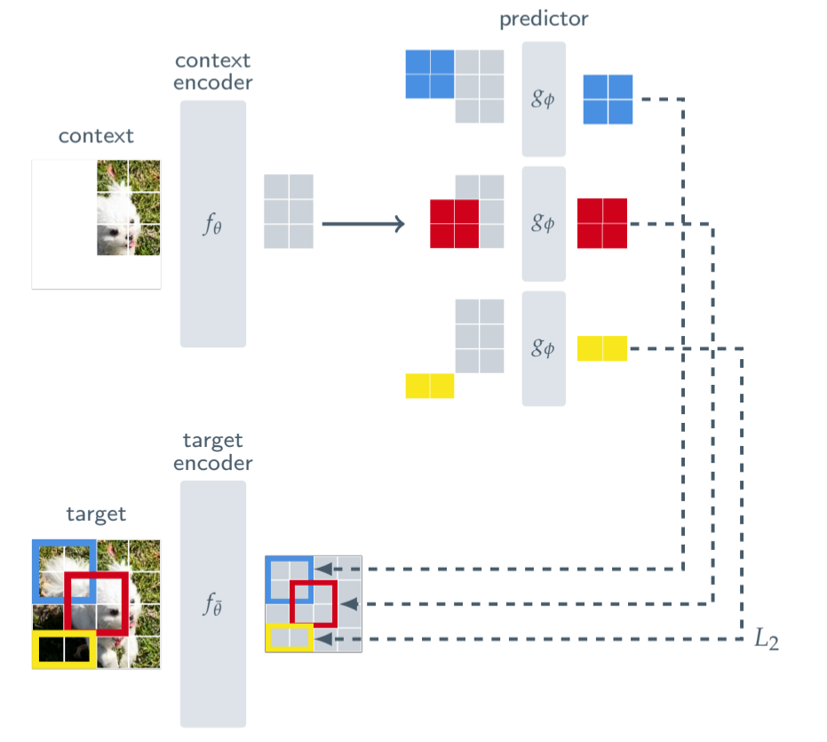
Source: Assran et al., 2023, Self-Supervised Learning from Images with a Joint-Embedding Predictive Architecture, Figure 3.

Context encoder

The context encoder takes the visible part of the input and turns it into an embedding, which we will call s_x. 

In I-JEPA, this is a ViT-Huge/14 with roughly 632 million parameters that only looks at the image patches it is allowed to see.

For a video, the visible part, this could be most of the clip, with a few regions blanked out. 

Going back to our paused ball video example earlier, the context encoder is you looking at the first half and noting “ball is moving right, slowing down” without writing down every pixel.

Target encoder

The target encoder looks at the hidden part (what is under the sticky notes) and produces the embedding we want to predict, s_y. 

It has the same design as the context encoder, but there is a twist: it is not trained directly.

Think about it: if both encoders were trained the same way, there is a chance that both models (via backpropagation) would converge to the same solution.

Instead, its weights are a slow-moving average of the context encoder’s weights, called an exponential moving average (EMA). 

Please don’t worry about the name; the idea is just that the teacher copies a tiny bit of the student’s latest knowledge after every lesson, so the teacher improves too, just much more slowly. We will see why this matters in the section below.

Predictor

The predictor takes s_x, plus a “note” about where the hidden part is (such as “top-left corner”), and outputs its guess for s_y. 

In I-JEPA, the predictor is a narrow ViT that is much smaller than the encoders, and this is on purpose, as we want the encoders to do most of the learning.

Think of it this way. If the context encoder is “what I can see” and the target encoder is “what is actually there”, then the predictor is “what I think is there”. 

The whole system learns by closing the gap between those last two.

The training signal

The loss is just the distance between the predictor’s guess and the target encoder’s embedding. In simple language, we can write loss = distance(predictor(s_x, where_the_target_is), s_y).

Here is a simplified PyTorch-style sketch of one training step. I have left out the masking code on purpose so that we can focus on the three parts:

import torch
import torch.nn.functional as F


def jepa_training_step(context_encoder, target_encoder, predictor,
                       optimizer, visible_patches, hidden_patches,
                       hidden_positions, ema_momentum=0.996):
    # 1. The "student" looks at the visible part
    s_x = context_encoder(visible_patches)

    # 2. The "teacher" looks at the hidden part (no gradients here)
    with torch.no_grad():
        s_y = target_encoder(hidden_patches)

    # 3. The student guesses the teacher's embedding
    s_y_pred = predictor(s_x, hidden_positions)

    # 4. Compare the two embeddings (no pixels involved)
    loss = F.smooth_l1_loss(s_y_pred, s_y)

    optimizer.zero_grad()
    loss.backward()
    optimizer.step()

    # 5. The teacher slowly copies the student (EMA update)
    with torch.no_grad():
        for p_teacher, p_student in zip(target_encoder.parameters(),
                                        context_encoder.parameters()):
            p_teacher.mul_(ema_momentum).add_((1 - ema_momentum) * p_student)

    return loss.item()

Please notice that there is no decoder anywhere in this code. 

In my world models article, the VAE needed a decoder to rebuild each CarRacing frame, and that decoder was often the most expensive part of a generative model. 

JEPA does not have one, which is a big reason the I-JEPA paper could train a ViT-Huge/14 on ImageNet using 16 A100 GPUs in under 72 hours.

The collapse problem and how JEPA solves it

But now here is the catch. Let’s go back to our classroom game and imagine a lazy student who writes “a thing” under every sticky note.

If the teacher also starts writing “a thing” for everything, the two descriptions match perfectly, and the student gets full marks without learning anything at all.

This is called representation collapse, and is what I mentioned briefly before. 

In a neural network, it happens when both encoders output the same embedding for every input, which makes the loss zero and the model useless.

The classic fix comes from contrastive learning. 

Methods such as SimCLR and CLIP also show the model negative pairs (“these two images are different, so their embeddings must be far apart”), which stops everything from being squashed into one point. 

Now this does work, but it usually needs very large batches (for example, SimCLR used batch sizes of up to 8,192) and hand-designed tricks such as random crops and color changes.

JEPA avoids negatives entirely by making the student and teacher different on purpose:

• Stop-gradient: the loss never updates the teacher (target encoder) directly, so the model cannot cheat by moving both embeddings to the same spot.
• Slow teacher (EMA): the teacher changes slowly, which gives the student a stable target to chase.
• Predictor on one side only: only the student has a predictor, which breaks the symmetry between the two encoders (asymmetric architecture).

I want to be clear that this design is partly trial and error. 

It works very well in practice (it was borrowed from earlier methods such as BYOL), but still, there is no clean proof of why it avoids collapse, and a badly tuned EMA can still break training.

LeJEPA’s theoretical advance (2025)

This is the gap that LeJEPA, published in November 2025 by Randall Balestriero and Yann LeCun, set out to close. 

The paper shows that the best shape for JEPA embeddings is an isotropic Gaussian. In simple terms, if you plotted all the embeddings, they should form an even, round cloud spread out in every direction, not a squashed line or a single dot.

The authors then add a new loss term called Sketched Isotropic Gaussian Regularization (SIGReg), which keeps checking that the embeddings still look like that round cloud. 

A collapsed model (all embeddings on one dot) can never pass this check, so collapse is prevented by design. According to the paper, LeJEPA:

• Drops the stop-gradient and the slow-teacher (EMA) setup
• Has only one trade-off hyperparameter to tune
• Needs roughly 50 lines of code
• Reaches 79% accuracy on ImageNet-1K with a ViT-H/14 (using a simple linear classifier on top of the frozen model)

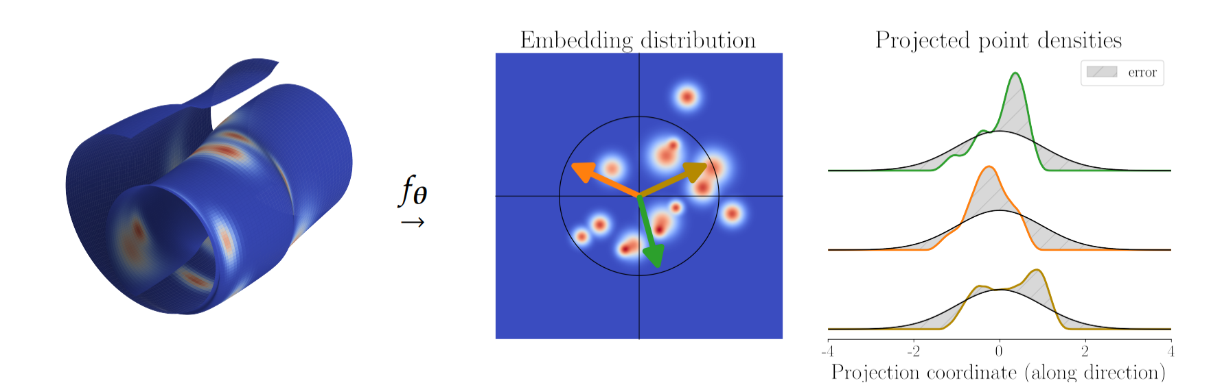
Source: Balestriero and LeCun, 2025, LeJEPA: Provable and Scalable Self-Supervised Learning Without the Heuristics, Figure 2.

If you want to try this yourself (and I would recommend it), the official repository can be installed with pip install lejepa and this SIGReg loss can be added to an existing training script.

Latent variables and planning under uncertainty

The real world is not always predictable. If you push a cup towards the edge of a table, it might stop, tip over, or slide off, and a single fixed prediction cannot cover all three.

In 2022, LeCun’s paper handles this by giving the predictor one more input, a latent variable z. 

I like to think of z as a dial, where each setting of the dial gives a different possible future, so turning it lets the model describe a whole set of plausible outcomes. 

If this sounds familiar, it is the same job the mixture-density network did in the MDN-RNN from the world models article, except that now it happens in embedding space.

This is also what turns JEPA from a model that understands into a model that actually can plan. 

See, once the predictor also takes an action as input, the model can answer “what will the world look like if I do this?”, and V-JEPA 2-AC uses exactly this idea to plan robot movements (we will see this in the next section)

The JEPA Model Family (2023-2026)

Now, let's talk about the entire JEPA Model Family.

It is a series of models, mostly from Meta FAIR, that all use the same context encoder, target encoder, and predictor architecture on different types of data. 

Each new model keeps the core idea and changes what the “visible part” and “hidden part” are. Let’s go through them in the order they came out.

I-JEPA (CVPR 2023)

I-JEPA, from Mahmoud Assran and colleagues, was the first time JEPA went from an idea in a paper to a working image model. 

It takes one large visible block of an image and predicts the embeddings of 4 hidden blocks elsewhere in the same image (exactly our sticky-note game).

What I like most about I-JEPA is that it needs no hand-made tricks. 

Contrastive methods such as SimCLR and DINO rely on randomly cropping, blurring, and recoloring images to learn, while I-JEPA only hides parts of the image. 

The code is on GitHub, and the model is also available in the Hugging Face transformers library.

This is a very straightforward paper to read, and I would recommend starting from here.

V-JEPA (2024)

V-JEPA, released by Adrien Bardes and colleagues in February 2024 (published in TMLR and presented at ICLR 2025), took the same idea to video. 

It hides regions across both space and time (for example, the bottom-right corner of the next few frames) and predicts their embeddings, with no labels, no text, and no negative examples.

It was trained on 2 million videos from public datasets.

It did really well on Something-Something-v2 (72.2%), which is a dataset that checks whether a model understands motion, such as “pushing something from left to right”, instead of just recognizing objects.

V-JEPA 2 and V-JEPA 2-AC (2025)

V-JEPA 2, released in June 2025, is where JEPA really started to look like a world model. 

Meta trained it on over 1 million hours of internet video plus images, and it scored 77.3% on Something-Something v2 and set a new best result for predicting what people in kitchen videos would do next (Epic-Kitchens-100).

But here is the part I found the most exciting. V-JEPA 2-AC (the AC stands for action-conditioned). The team froze V-JEPA 2 and trained a new predictor on less than 62 hours of unlabeled robot video from the DROID dataset, so it learned how the embedding changes when a robot arm moves. 

They then put it on Franka robot arms in two different labs it had never seen, where it picked up and placed objects using only a photo of the goal, with no extra data from those labs and no task-specific rewards.

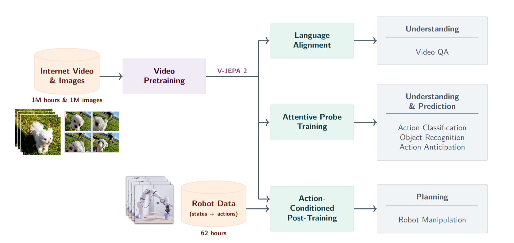
Source: Assran et al., 2025, V-JEPA 2: Self-Supervised Video Models Enable Understanding, Prediction and Planning, Figure 1. Licensed under CC BY 4.0.

Now you might ask the question, how does it plan?

At each step, the robot tries out many possible action sequences in its head, uses the predictor to imagine where each one ends up, and picks the one whose final embedding is closest to the embedding of the goal photo. 

This is the same see, remember, act loop from the original 2018 World Models paper, except that the imagining now happens entirely in JEPA’s embedding space.

If you want to experiment with it yourself, the weights are available through torch.hub using this code:

import torch

# Load a pretrained V-JEPA 2 video encoder (ViT-L)
vjepa2_encoder = torch.hub.load("facebookresearch/vjepa2", "vjepa2_vit_large")

# Load the action-conditioned world model used for robot planning
ac_encoder, ac_predictor = torch.hub.load("facebookresearch/vjepa2",
                                          "vjepa2_ac_vit_giant")

V-JEPA 2.1 (March 2026)

V-JEPA 2.1, released on March 16, 2026, by Lorenzo Mur-Labadia and colleagues, focuses on fine detail. 

V-JEPA 2 was great at understanding a whole scene, but less precise about small things, such as the exact edge of an object or how far away it is, which matters a lot when a robot gripper is trying to grab something.

The new method makes four changes:

• A dense predictive loss, meaning the visible parts are scored as well as the hidden parts, not just the hidden parts
• Deep self-supervision, which checks the model’s answers at several layers inside the encoder instead of only the last one
• Multimodal tokenizers, so one model can train on both images and video
• Scaling up both the model size and the training data

Based on what the authors have stated, V-JEPA 2.1 gives a 20-point improvement in real-robot grasping success over V-JEPA 2-AC. 

The pretrained models, from ViT-B up to a ViT-G (“gigantic”) version, are in the same facebookresearch/vjepa2 repository.

VL-JEPA (December 2025)

VL-JEPA, from Delong Chen, Mustafa Shukor, and colleagues at Meta FAIR (accepted at ICLR 2026), brings JEPA to vision and language. 

A typical vision language model (VLM) writes its answer word by word, while VL-JEPA predicts the embedding of the answer and only turns it into words when it actually needs to.

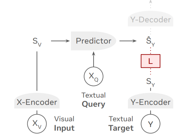
Source: Chen et al., 2025, VL-JEPA: Joint Embedding Predictive Architecture for Vision-language, Figure 1. Licensed under CC BY 4.0.

It is trained with an InfoNCE-style contrastive loss, so in that sense it plays a similar role to CLIP. 

The difference is that VL-JEPA predicts the text embedding from a video and a question, instead of just matching two embeddings, and the authors reported better results than a standard word-by-word VLM with 50% fewer trainable parameters.

LeJEPA (November 2025)

LeJEPA is a bit different from the rest of the family, as it is mainly a theory paper with a training recipe attached. 

As we covered in the collapse section, Randall Balestriero and Yann LeCun replaced the slow-teacher trick with SIGReg, a single loss term with proven guarantees, and released it as a small Python package.

Summary table

I have also created a table to see the whole family in one place:

JEPA as a General Self-Supervised Recipe

JEPA has turned into a general recipe for self-supervised learning, because it works on any data where you can hide one part and predict it from another part. 

Hopefully, you will agree with me that this is where things get really interesting as researchers outside Meta have now used it on sound, 3D scans, molecules, sensor readings, and even brain signals.

In my opinion, the best way to see this is to look at what the visible part and hidden part are in each case:

If you work with structured or time-based data, a few of these are also worth looking at:

• MTS-JEPA (2026) from Yanan He and colleagues looks at a time series at several zoom levels at once, which helps it predict anomalies before they fully show up.
• LaT-PFN (2024) from Stijn Verdenius and colleagues combines JEPA with prior-fitted networks so it can forecast a brand-new series without retraining. If you read my article on tabular foundation models, this is a close cousin of TabPFN.
• T-JEPA (2024) from Hugo Thimonier and colleagues uses JEPA on tables without any augmentations. Watch out for the name, as a different paper also called T-JEPA (Lihuan Li and colleagues, 2024) uses it for comparing movement trajectories instead.
• S-JEPA (2024) from Pierre Guetschel and colleagues learns from EEG brain signals and works across datasets recorded with different electrode layouts, which has been a long-standing headache in brain-computer interfaces.

In short, JEPA gives you the architecture, and domain experts bring the “what do we hide?” part. 

If you can explain what hiding part of your data means for your problem, you can probably train a JEPA on it.

LeCun’s Autonomous Intelligence Blueprint: Where JEPA Fits

In LeCun’s blueprint, JEPA is the world model: one of six parts of a bigger system designed to see, predict, plan and act on its own. 

This bigger picture is what the 2022 paper was really about, and I think it explains why Meta (and now LeCun’s own startup, AMI Labs) has been betting on JEPA for so long.

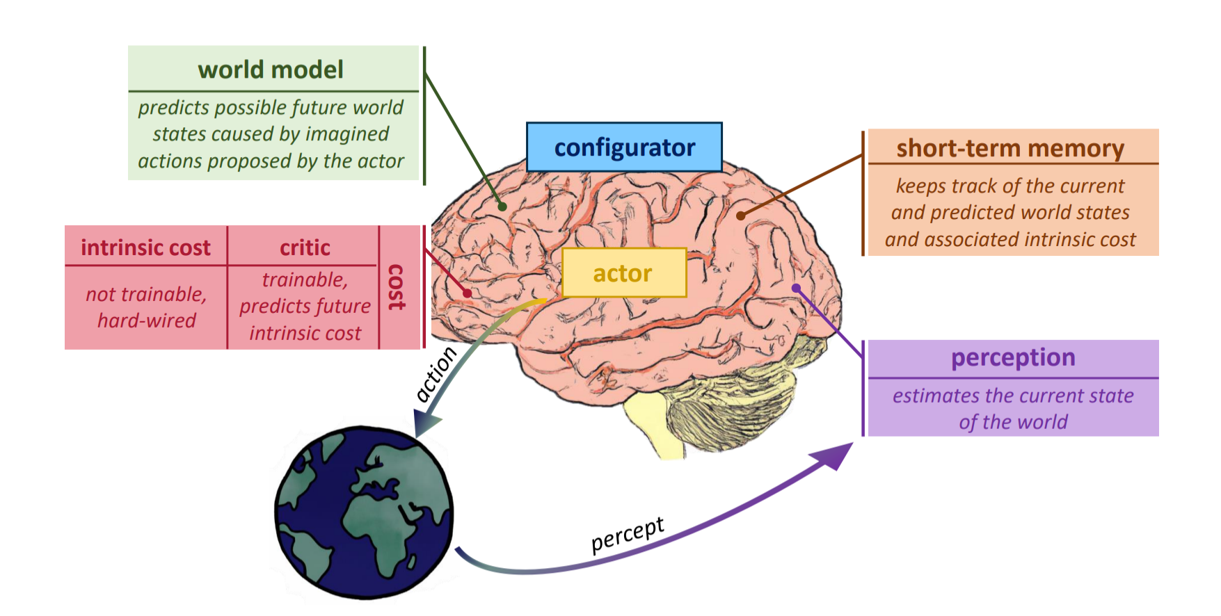
Source: Dawid and LeCun, 2023, Introduction to Latent Variable Energy-Based Models: A Path Towards Autonomous Machine Intelligence, Figure 1, which presents the architecture proposed in LeCun, 2022, A Path Towards Autonomous Machine Intelligence. The drawings were generated by DALL-E 2, as noted in the paper.

The six modules

To keep this section simple, let's imagine a robot whose job is to just clear a kitchen table. Here is what each module does:

1. Configurator: The “manager” that sets up the other modules for the task at hand. For clearing the table, it tells them to pay attention to plates and cups.
2. Perception: Turns raw sensor data (camera images, joint positions) into a summary of what the world looks like right now. In a JEPA system, this is the context encoder.
3. World model: Predicts how that summary will change after a sequence of actions. This is where JEPA sits, and it is the most complex part of the design.
4. Cost module: Scores how “bad” a situation is. It has fixed rules (for example, “do not drop the plate”) plus a learned critic that estimates future cost.
5. Actor: Comes up with possible action sequences and searches for the one the world model predicts will have the lowest cost.
6. Short-term memory: Keeps track of recent states, predictions, and costs, very similar to the memory component in Ha and Schmidhuber’s world model.

LeCun also suggests stacking JEPAs on top of each other, which he calls a hierarchical JEPA (H-JEPA). 

The lower level predicts short, detailed changes (“the gripper moves 2 cm”), while the higher level predicts long, big-picture changes (“the plate ends up in the sink”).

The planning loop

If we put these together, these modules run in a loop that LeCun calls “Mode-2” reasoning, meaning slow and careful planning (as opposed to fast, automatic “Mode-1” reactions):

1. Perceive: Turn the current camera image into an embedding.
2. Imagine: The actor proposes a few action sequences, and the JEPA world model predicts the future embedding for each one.
3. Score: The cost module rates each imagined future.
4. Act: The robot carries out only the first action of the best sequence.
5. Repeat: It looks at the new situation and plans again, which fixes small prediction mistakes along the way.

If you have read the V-JEPA 2-AC paper, this might sound familiar because V-JEPA 2-AC already does a simpler version of this loop. 

Its “cost” is just the distance between the predicted embedding and the embedding of the goal photo, and its “actor” is a trial-and-error search over candidate actions.

Current status

But I want to be clear about how far along all of this actually is. V-JEPA 2-AC shows that the perceive, imagine, score, and act loop works for short tasks such as picking and placing objects, in labs that the robot had never seen.

The full blueprint, though, with a learned configurator, a trained critic, and a deep H-JEPA stack, is still a research roadmap and not something we can download. 

LeCun left Meta in late 2025 to found AMI Labs, which raised $1.03 billion in March 2026 to chase this vision, but has not shipped a model yet.

Where JEPA Fits in the 2026 AI Stack

Another question you might be asking is where JEPA actually fits in the entire AI stack?

See in 2026, JEPA fits into the AI stack as the layer that predicts and plans in the physical world, working next to LLMs and VLMs rather than replacing them. 

A lot of headlines describe JEPA as LeCun’s big bet to kill off LLMs, and I understand why (because he has been very vocal about their limits), but that framing misses how the two are actually being used together.

The simplest way I can put it is that they are good at very different jobs:

And we can already see this split in real systems:

• V-JEPA 2 was connected to a language model to answer questions about videos, scoring 84.0 on the PerceptionTest benchmark at the 8 billion parameter scale. JEPA does the seeing, and the LLM does the talking.
• VLA-JEPA (2026) pairs a vision-language-action model with a JEPA world model, so the robot’s policy can use predicted futures when choosing what to do.
• VL-JEPA goes one step further and moves part of the language side itself into embedding space, so words are only generated when they are actually needed.

This is the same setup behind the wider physical AI wave I covered in my articles on embodied AI and vision-language-action (VLA) models. 

In those systems, an LLM or VLM handles the language and instructions, and a world model (more and more often a JEPA-style one) handles the physics.

In short, JEPA and LLMs are a team. The LLM tells the robot what to do, and JEPA helps it work out what will happen if it does it.

Final Thoughts

Now, remember the ball flying across the park at the start of this article? JEPA is built around the idea that a good model should care about where the ball lands, not how every leaf moves. 

It does this by predicting summaries (embeddings) instead of pixels, using a context encoder, a target encoder, and a predictor, and avoids collapse through a clever student-and-slow-teacher setup (or, since LeJEPA, through a proven regularizer).

In just 4 years, the family has gone from a position paper to I-JEPA, V-JEPA, V-JEPA 2-AC controlling real robot arms and V-JEPA 2.1, with spin-offs now covering audio, 3D, molecules, time series, and brain signals. 

What really shocks me personally is how much progress that is for an idea many people brushed off as contrarian back in 2022.

If you want to build the deep learning foundations needed to work with architectures like JEPA, I recommend the Deep Learning in Python track. And for the language side of the stack, the Developing Large Language Models track is a great next step.