

What Are Transformers?
Transformers were first developed to solve the problem of sequence transduction, or neural machine translation, which means they are meant to solve any task that transforms an input sequence to an output sequence. This is why they are called “Transformers”.
But let’s start from the beginning.
A Simple Definition
A transformer model is a neural network that learns the context of sequential data and generates new data out of it.
To put it simply:
A transformer is a type of artificial intelligence model that learns to understand and generate human-like text by analyzing patterns in large amounts of text data.
Transformers are a current state-of-the-art NLP model and are considered the evolution of the encoder-decoder architecture. However, while the encoder-decoder architecture relies mainly on Recurrent Neural Networks (RNNs) to extract sequential information, Transformers completely lack this recurrency.
So, how do they do it?
They are specifically designed to comprehend context and meaning by analyzing the relationship between different elements, and they rely almost entirely on a mathematical technique called attention to do so.
Image by the author.
Historical Context
Transformers were introduced by Google researchers in the 2017 paper "Attention is All You Need". The code was released in TensorFlow’s Tensor2Tensor package, and the Harvard NLP group followed with an annotated guide to the paper in PyTorch. You can also learn how to implement a Transformer from scratch in our separate tutorial.
Within a year, Google’s BERT and OpenAI’s GPT-1 showed that a transformer pre-trained on unlabeled text could be fine-tuned for almost any language task. GPT-3 followed in 2020, and Stanford researchers coined the term “foundation models” for this new class of models.
Since then, things have moved fast: open-weight models like Meta’s Llama (2023), multimodal models like GPT-4o (2024), reasoning models like OpenAI’s o1 and DeepSeek-R1 (late 2024 to early 2025), and agentic models like GPT-5 (2025) and GPT-6 Astra (2026). The models whose designs are public are all still transformers. For the full story, see our history of large language models.
The Shift From RNN Models to Transformers
When the Transformer was introduced, recurrent neural networks (RNNs) and their long short-term memory (LSTM) variant were the go-to models for sequential data. They process the input one element at a time, which causes two main problems:
- Slow training: each step waits for the previous one, so RNNs can’t use the parallel computation GPUs are built for.
- Forgetting over long distances: information is passed along step by step, and the longer the chain, the more likely it gets lost.
Transformers kept the encoder-decoder idea from RNNs but replaced recurrence with attention, which fixes both problems: every word can attend directly to any other word, no matter how far apart, and the whole sequence is processed in parallel.
Next, let’s take a look at how transformers work.
How Does the Transformer Architecture Work?
Originally devised for sequence transduction or neural machine translation, transformers excel in converting input sequences into output sequences. It is the first transduction model relying entirely on self-attention to compute representations of its input and output without using sequence-aligned RNNs or convolution. The main core characteristic of the Transformers architecture is that they maintain the encoder-decoder model.
If we start considering a Transformer for language translation as a simple black box, it would take a sentence in one language, English for instance, as an input and output its translation in Spanish.
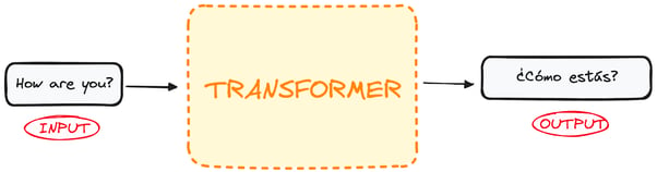
Image by the author.
If we dive a little bit, we observe that this black box is composed of two main parts:
- The encoder takes in our input and outputs a matrix representation of that input. For instance, the English sentence “How are you?”
- The decoder takes in that encoded representation and iteratively generates an output. In our example, the translated sentence “¿Cómo estás?”
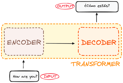
Image by the author. Global structure of Encoder-Decoder.
However, both the encoder and the decoder are actually a stack with multiple layers (same number for each). All encoders present the same structure, and the input gets into each of them and is passed to the next one. All decoders present the same structure as well and get the input from the last encoder and the previous decoder.
The original architecture consisted of 6 encoders and 6 decoders, but we can replicate as many layers as we want. So let’s assume N layers of each.
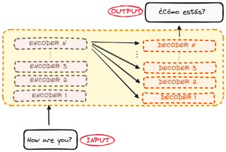
Image by the author. Global structure of Encoder-Decoder. Multiple Layers.
So now that we have a generic idea of the overall Transformer architecture, let’s focus on both Encoders and Decoders to understand better their working flow:
How Does the Transformer Encoder Work?
The encoder is a fundamental component of the Transformer architecture. The primary function of the encoder is to transform the input tokens into contextualized representations. Unlike earlier models that processed tokens independently, the Transformer encoder captures the context of each token with respect to the entire sequence.
Its structure composition consists as follows:
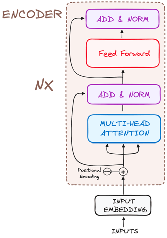
Image by the author. Global structure of Encoders.
So let’s break its workflow into its most basic steps:
Step 1: Input embeddings
The embedding only happens in the bottom-most encoder. First, a tokenizer splits the text into tokens, which are words or pieces of words, and each token is mapped to a learned vector called an embedding. Tokens with related meanings end up with similar vectors.
All the encoders receive a list of vectors, each with 512 dimensions in the original paper (dmodel = 512). In the bottom encoder, that would be the word embeddings, but in other encoders, it would be the output of the encoder that’s directly below them.
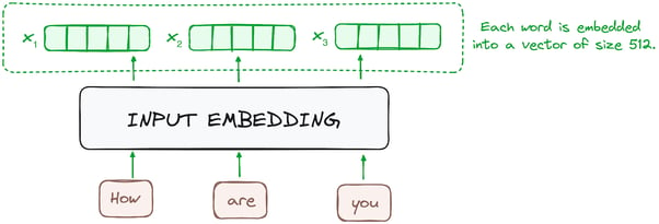
Image by the author. Encoder’s workflow. Input embedding.
Step 2: Positional encoding
Since Transformers do not have a recurrence mechanism like RNNs, they use positional encodings added to the input embeddings to provide information about the position of each token in the sequence. This allows them to understand the position of each word within the sentence.
To do so, the researchers suggested employing a combination of various sine and cosine functions to create positional vectors, enabling the use of this positional encoder for sentences of any length.
In this approach, each dimension is represented by unique frequencies and offsets of the wave, with the values ranging from -1 to 1, effectively representing each position.
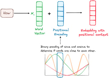
Image by the author. Encoder’s workflow. Positional encoding.
Step 3: Stack of encoder layers
The Transformer encoder consists of a stack of identical layers (6 in the original Transformer model).
The encoder layer serves to transform all input sequences into a continuous, abstract representation that encapsulates the learned information from the entire sequence. This layer comprises two sub-modules:
- A multi-headed attention mechanism.
- A fully connected network.
Additionally, it incorporates residual connections around each sublayer, which are then followed by layer normalization.
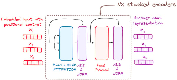
Image by the author. Encoder’s workflow. Stack of Encoder Layers
Step 3.1: Multi-headed self-attention mechanism
In the encoder, the multi-headed attention utilizes a specialized attention mechanism known as self-attention. This approach enables the models to relate each word in the input with other words. For instance, in a given example, the model might learn to connect the word “are” with “you”.
This mechanism allows the encoder to focus on different parts of the input sequence as it processes each token. It computes attention scores based on:
- A query is a vector that represents a specific word or token from the input sequence in the attention mechanism.
- A key is also a vector in the attention mechanism, corresponding to each word or token in the input sequence.
- Each value is associated with a key and is used to construct the output of the attention layer. When a query and a key match well, which basically means that they have a high attention score, the corresponding value is emphasized in the output.
This first Self-Attention module enables the model to capture contextual information from the entire sequence. Instead of performing a single attention function, queries, keys and values are linearly projected h times. On each of these projected versions of queries, keys and values the attention mechanism is performed in parallel, each producing an output of dv dimensions (64 in the original paper, where h = 8).
The detailed architecture goes as follows:
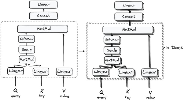
Matrix multiplication (MatMul): dot product of query and key
Once the query, key, and value vectors are passed through a linear layer, a dot product matrix multiplication is performed between the queries and keys, resulting in the creation of a score matrix.
The score matrix establishes the degree of emphasis each word should place on other words. Therefore, each word is assigned a score in relation to other words within the same time step. A higher score indicates greater focus.
This process effectively maps the queries to their corresponding keys.
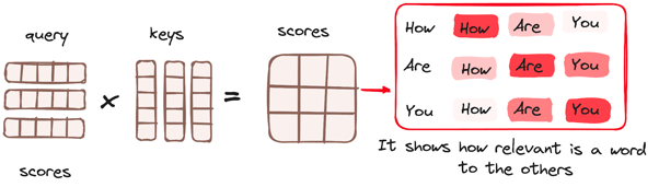
Image by the author. Encoder’s workflow. Attention mechanism - Matrix Multiplication.
Reducing the magnitude of attention scores
The scores are then scaled down by dividing them by the square root of the dimension of the query and key vectors. This step is implemented to ensure more stable gradients, as the multiplication of values can lead to excessively large effects.
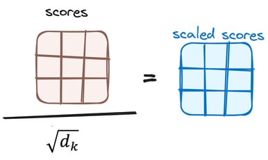
Image by the author. Encoder’s workflow. Reducing the attention scores.
Applying softmax to the adjusted scores
Subsequently, a softmax function is applied to the adjusted scores to obtain the attention weights. This results in probability values ranging from 0 to 1. The softmax function emphasizes higher scores while diminishing lower scores, thereby enhancing the model's ability to effectively determine which words should receive more attention.
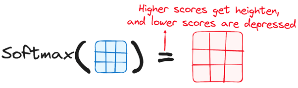
Image by the author. Encoder’s workflow. Softmax adjusted scores.
Combining softmax results with the value vector
The following step of the attention mechanism is that weights derived from the softmax function are multiplied by the value vector, resulting in an output vector.
Words with high softmax weights dominate the result, while words with weights near 0 contribute almost nothing. Finally, this output vector is fed into a linear layer for further processing.
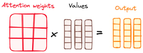
Image by the author. Encoder’s workflow. Combining Softmax results with the value vector.
And we finally get the output of the Attention mechanism!
The word “multi-head” comes from running this process several times in parallel. Before attention starts, the queries, keys, and values are split into h smaller sets called heads, and each head runs the steps above on its own slice.
The head outputs are concatenated and passed through a final linear layer. Because each head learns its own projections, different heads can pick up different relationships, such as which noun a pronoun refers to or which words sit next to each other.
For a deeper understanding of the attention mechanism, see our tutorial on multi-head attention in Transformers.
Step 3.2: Normalization and residual connections
Each sub-layer in an encoder layer is followed by a normalization step. Also, each sub-layer output is added to its input (residual connection) to help mitigate the vanishing gradient problem, allowing deeper models. This process will be repeated after the Feed-Forward Neural Network too.
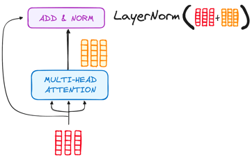
Image by the author. Encoder’s workflow. Normalization and residual connection after Multi-Head Attention.
Step 3.3: Feed-forward neural network
Next, the output passes through a position-wise feed-forward network: 2 linear layers with a ReLU activation between them, applied to each token separately. In the original paper, the inner layer has 2,048 dimensions, 4 times the model width of 512.
As with attention, the network’s input is added back to its output (a residual connection), and the result is normalized.
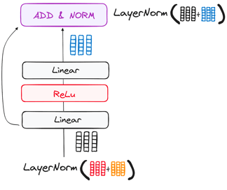
Image by the author. Encoder’s workflow. Feed-Forward Neural Network sub-layer.
Step 4: Output of the encoder
The output of the final encoder layer is a set of vectors, each representing the input sequence with a rich contextual understanding. This output is then used as the input for the decoder in a Transformer model.
This careful encoding paves the way for the decoder, guiding it to pay attention to the right words in the input when it's time to decode.
Stacking N encoder layers lets each layer build on the representations of the one below it. The original model used N = 6; BERT-Base uses 12 and BERT-Large 24.
How Does the Transformer Decoder Work?
The decoder generates the output sequence. Its layers mirror the encoder’s with 1 addition: each layer has 2 multi-head attention sub-layers instead of 1, followed by a position-wise feed-forward network, with a residual connection and layer normalization around every sub-layer.
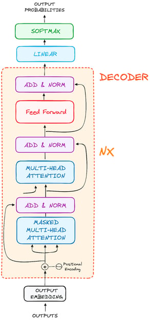
Image by the author. Global structure of Decoders.
These components function in a way akin to the encoder's layers, yet with a twist: each multi-headed attention layer in the decoder has its unique mission.
The final of the decoder's process involves a linear layer, serving as a classifier, topped off with a softmax function to calculate the probabilities of different words.
The Transformer decoder has a structure specifically designed to generate this output by decoding the encoded information step by step.
The decoder works autoregressively: it starts with a start-of-sequence token and, at every step, takes the tokens it has generated so far as input, together with the encoder’s output.
It stops when it generates an end-of-sequence token.
Step 1: Output embeddings
At the decoder's starting line, the process mirrors that of the encoder. Here, the input first passes through an embedding layer.
Step 2: Positional encoding
Following the embedding, again just like the encoder, the input passes by the positional encoding layer. This sequence is designed to produce positional embeddings.
These positional embeddings then go into the first multi-head attention layer of the decoder, where the attention scores for the decoder’s own input are computed.
Step 3: Stack of decoder layers
The decoder consists of a stack of identical layers (6 in the original Transformer model). Each layer has three main sub-components:
Step 3.1: Masked self-attention mechanism
This is similar to the self-attention mechanism in the encoder but with a crucial difference: it prevents positions from attending to subsequent positions, which means that each word in the sequence isn't influenced by future tokens.
For instance, when the attention scores for the word “Cómo” are being computed, it’s important that “Cómo” doesn’t get a peek at “estás”, which is a subsequent word in the output sequence.
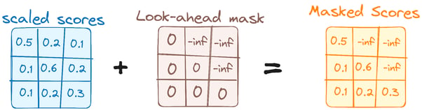
Image by the author. Decoder’s workflow. First Multi-Head Attention Mask.
This masking ensures that the predictions for a particular position can only depend on known outputs at positions before it.
Step 3.2: Encoder-decoder attention (cross-attention)
The second attention sub-layer connects the decoder to the encoder. Here, the queries come from the decoder’s masked self-attention output, while the keys and values come from the encoder’s final output.
This lets every position in the decoder attend over all positions in the input sentence, so when generating “estás,” the decoder can focus on “are you.” The result then goes through the feed-forward sub-layer.
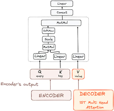
Image by the author. Decoder’s workflow. Encoder-Decoder Attention.
Step 3.3: Feed-forward neural network
Similar to the encoder, each decoder layer includes a fully connected feed-forward network, applied to each position separately and identically.
Step 4: Linear classifier and softmax
The journey of data through the transformer model culminates in its passage through a final linear layer, which functions as a classifier.
The size of this classifier corresponds to the total number of classes involved (number of words contained in the vocabulary). For instance, in a scenario with 1000 distinct classes representing 1000 different words, the classifier's output will be an array with 1000 elements.
This output is then introduced to a softmax layer, which transforms it into a range of probability scores, each lying between 0 and 1. The token with the highest probability is the model’s best guess for the next word. Greedy decoding always picks it; most chat models instead sample from the distribution, with a temperature setting that controls how much randomness is allowed.
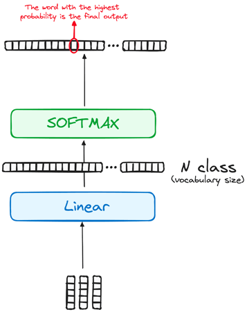
Image by the author. Decoder’s workflow. Transformer’s final output.
Normalization and residual connections
Each sub-layer (masked self-attention, encoder-decoder attention, feed-forward network) is followed by a normalization step, and each also includes a residual connection around it.
Output of the decoder
The final layer's output is transformed into a predicted sequence, typically through a linear layer followed by a softmax to generate probabilities over the vocabulary.
The decoder, in its operational flow, incorporates the freshly generated output into its growing list of inputs, and then proceeds with the decoding process. This cycle repeats until the model predicts a specific token, signaling completion.
Like the encoder, the decoder is a stack of N identical layers (6 in the original model), each building on the output of the layer below and on the encoder’s output. Deeper stacks let different layers and heads capture different attention patterns.
The final architecture looks like this (from the original paper):
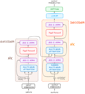
Image by the author. Original structure of Transformers.
To better understand this architecture, I recommend trying to apply a Transformer from scratch by following this tutorial to build a transformer with PyTorch.
Encoder-Only, Decoder-Only, and Encoder-Decoder Transformers
Transformer models fall into 3 families, depending on which half of the original architecture they keep. The choice decides what a model is good at: encoders read, decoders write, and encoder-decoders map one sequence onto another.
| Family | What it keeps | Attention | Pre-training task | Typical uses | Examples |
|---|---|---|---|---|---|
| Encoder-only | Encoder stack | Bidirectional: every token sees every token | Fill in masked tokens | Classification, search embeddings, named entity recognition | BERT, RoBERTa |
| Decoder-only | Decoder stack, without cross-attention | Causal: each token sees only earlier tokens | Predict the next token | Chat, code generation, agents | GPT-3, Llama, Gemini |
| Encoder-decoder | Both stacks | Bidirectional encoder, causal decoder, plus cross-attention | Map an input sequence to an output sequence | Translation, summarization, speech recognition | Original Transformer, T5, Whisper |
Most LLMs released since GPT-3 are decoder-only. Next-token prediction works on any raw text, so training data is plentiful, and one model can handle translation, summarization, and question answering by treating each as text continuation.
Which Models Use the Transformer Architecture?
BERT
BERT (Bidirectional Encoder Representations from Transformers), released as open source by Google in 2018, is an encoder-only transformer. Instead of predicting the next word, it was pre-trained to fill in masked words using the context on both sides, which made it stronger at understanding tasks than the left-to-right models of the time.
By understanding context from all sides of a word, BERT outperformed previous models in tasks like question-answering and understanding ambiguous language. Its core uses Transformers, connecting each output and input element dynamically.
BERT was pre-trained on English Wikipedia and the BooksCorpus dataset, and Google added it to Search in 2019 to better interpret natural-language queries. It set off a race to build larger pre-trained language models.
To know more about BERT, you can go check our separate article that introduces the BERT model.
LaMDA
LaMDA (Language Model for Dialogue Applications) is a Transformer-based model developed by Google, designed specifically for conversational tasks, and launched during the 2021 Google I/O keynote. They are designed to generate more natural and contextually relevant responses, enhancing user interactions in various applications.
LaMDA's design enables it to understand and respond to a wide range of topics and user intents, making it ideal for applications in chatbots, virtual assistants, and other interactive AI systems where a dynamic conversation is key.
Google later replaced LaMDA in its Bard chatbot with PaLM 2, and then Gemini, but LaMDA was one of the first transformer models trained specifically on dialogue.
If you are interested in further understanding the LaMDA models, you can get a better understanding with our article on LaMDA.
GPT and ChatGPT
GPT and ChatGPT, developed by OpenAI, are advanced generative models known for their ability to produce coherent and contextually relevant text. GPT-1 was the first model launched in June 2018, and GPT-3, one of the most impactful models, was launched two years later in 2020.
These models are adept at a wide range of tasks, including content creation, conversation, language translation, and more. GPT's architecture enables it to generate text that closely resembles human writing, making it useful in applications like creative writing, customer support, and even coding assistance. ChatGPT, a variant optimized for conversational contexts, excels in generating human-like dialogue, enhancing its application in chatbots and virtual assistants.
OpenAI stopped publishing architecture details after GPT-3 (except for their open-weight gpt-oss models), but the family has kept growing, most recently with GPT-6 Astra in 2026.
Claude
Claude, developed by Anthropic, is a family of Transformer-based AI assistants designed with a focus on safety and helpfulness. Claude uses Constitutional AI (CAI), a training approach where the model is guided by a set of principles to produce helpful, harmless, and honest responses.
Claude 3 (released in 2024) introduced three model tiers, Haiku, Sonnet, and Opus, offering different trade-offs between speed and capability. The models excel at nuanced reasoning, following complex instructions, and maintaining context over long conversations (up to 200K tokens).
Anthropic has released new generations every few months since then. The current Claude 5 lineup includes Claude Fable 5.1 and Claude Opus 5.5, both released in 2026. Like OpenAI, Anthropic doesn’t publish its architecture details.
Other Variations
The number of transformer models has grown fast. Xavier Amatriain’s catalog of transformer models classifies dozens of them by architecture and training objective, and Stanford’s HELM benchmark evaluated 30 prominent language models side by side.
There is an increasing trend towards making these models open-source, with platforms like Hugging Face's model hub leading the way. Additionally, numerous Transformer-based models have been developed, each specialized for different NLP tasks, showcasing the model's versatility and efficiency in diverse applications.
You can learn more from all existing Foundation Models in a separate article, which talks about what they are and which ones are the most used.
How Have Transformers Changed Since 2017?
Since the original 2017 architecture, Transformers have evolved significantly to address limitations and expand to new domains.
How modern LLMs differ from the original Transformer
Today’s open-weight LLMs still follow the 2017 blueprint, but almost every component has been swapped for a variant that trains more stably or runs more cheaply. Meta documents most of these changes in its LLaMA and Llama 3 papers:
| Component | Original Transformer (2017) | Typical open-weight LLM today |
|---|---|---|
| Architecture | Encoder-decoder, 6 + 6 layers | Decoder-only, 32 layers (Llama 3 8B) to 126 layers (Llama 3 405B) |
| Model width | 512 | 4,096 (Llama 3 8B) to 16,384 (Llama 3 405B) |
| Position information | Fixed sine and cosine encodings added to the embeddings | Rotary position embeddings (RoPE) applied inside attention |
| Normalization | LayerNorm after each sub-layer (post-norm) | RMSNorm before each sub-layer (pre-norm) |
| Feed-forward activation | ReLU | SwiGLU |
| Attention heads | Multi-head attention, 8 heads | Grouped-query attention: several query heads share 1 key-value head (8 key-value heads in Llama 3) |
| Feed-forward layer | Dense | Dense, or mixture of experts (Llama 4, DeepSeek-V3) |
Vision Transformers (ViT)
Vision Transformers apply the self-attention mechanism to images by dividing them into patches and treating each patch as a token. This approach has proven highly effective for image classification, object detection, and image generation, often outperforming traditional CNNs on large datasets.
Multimodal Transformers
Modern models like GPT-5, Gemini 3, and Llama 4 process multiple input types (text, images, audio, video) within a single architecture. These multimodal Transformers use unified embedding spaces and cross-attention mechanisms to reason across different modalities simultaneously.
Efficient Transformers
The quadratic complexity of self-attention limits context length. Several innovations address this:
- Flash Attention: Computes exact attention in tiles that fit in the GPU’s fast on-chip memory, so memory use grows linearly with sequence length instead of quadratically
- Rotary Position Embeddings (RoPE): Encodes position information through rotation matrices, enabling better extrapolation to longer sequences
- Linear and sparse attention: Linformer and Performer approximate attention, and Longformer limits most tokens to a local window, bringing the cost down to O(n) for very long documents
- Mixture of Experts (MoE): Activates only a subset of parameters per token, enabling larger models with similar compute costs
Transformers vs. RNNs and CNNs
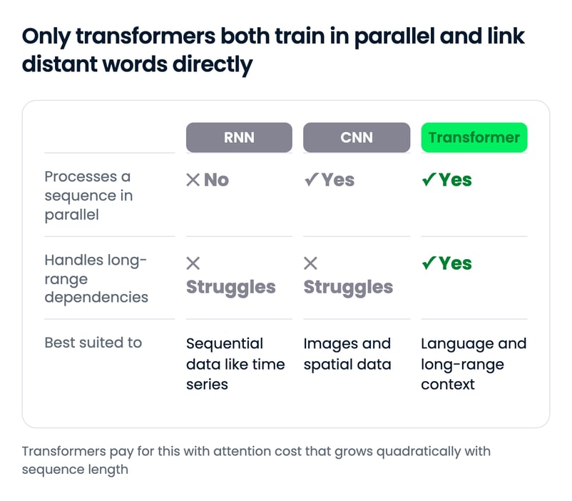
Transformers are usually compared with 2 other neural network building blocks: recurrent layers (RNNs) and convolutional layers (CNNs). Each suits a different kind of data.
Recurrent Layers
Recurrent Layers, a cornerstone of Recurrent Neural Networks (RNNs), excel in handling sequential data. This architecture's strength lies in its ability to perform sequential operations, crucial for tasks like language processing or time series analysis. In a Recurrent Layer, the output from a previous step is fed back into the network as input for the next step. This looping mechanism allows the network to remember previous information, which is vital in understanding context in a sequence.
However, as we have already discussed, this sequential processing has two main implications:
- It can lead to longer training times since each step depends on the previous one, making parallel processing challenging.
- They often struggle with long-term dependencies due to the vanishing gradient problem, where the network becomes less effective at learning from data points that are far apart in a sequence.
Transformer models differ significantly from architectures using recurrent layers as they lack recurrency. As we have seen before,the Transformer’s Attention layer addresses both problems, making them the natural evolution of RNNs for NLP applications.
Convolutional Layers
On the other hand, Convolutional Layers, the building blocks of Convolutional Neural Networks (CNNs), are renowned for their efficiency in processing spatial data like images.
These layers use kernels (filters) that scan over input data to extract features. The width of these kernels can be adjusted, allowing the network to focus on small or large features, depending on the task at hand.
While Convolutional Layers are exceptionally good at capturing spatial hierarchies and patterns in data, they face challenges with long-term dependencies. They do not inherently account for sequential information, making them less suitable for tasks that require understanding the order or context of a sequence.
This is why CNNs and Transformers are tailored for different types of data and tasks. CNNs dominate in the field of computer vision due to their efficiency in processing spatial information, while Transformers are the go-to choice for complex sequential tasks, especially in NLP, due to their ability to understand long-range dependencies.
Transformer Drawbacks and Limitations
Despite their success, Transformers have notable limitations:
- Quadratic complexity: Self-attention scales as O(n²) with sequence length, making very long context windows computationally expensive
- Memory requirements: Large models require significant GPU memory, limiting deployment options
- Training data requirements: Transformers typically need massive datasets to achieve strong performance
- Hallucination: Transformers predict likely tokens rather than look facts up, so they can state false information confidently. Reasoning models reduce this but don’t remove it
- Position encoding limitations: Standard positional encodings struggle to generalize to sequence lengths not seen during training
Research continues to address these limitations through architectural innovations likeFlash Attention, mixture-of-experts, and retrieval-augmented generation (RAG).
Final Thoughts
A transformer works by letting every token look at every other token through self-attention, then refining those representations through a stack of identical layers. That one design choice made training parallel on GPUs and solved the long-range memory problem that held back RNNs.
What strikes me most is how little the core has changed. A 2026 LLM swaps the positional encoding, the normalization, and the attention heads for cheaper variants, but you would still recognize the 2017 diagram in it. The open question is whether state space models and hybrids will take over long contexts, or whether kernels like FlashAttention keep attention’s quadratic cost affordable.
To put this into practice, build a Transformer with PyTorch in our step-by-step tutorial, or start with pretrained models in our introduction to Transformers and Hugging Face. If you’re keen to learn more, I recommend the Transformer Models with PyTorch course, or the Developing Large Language Models track for the full path.
FAQs
How does the transformer architecture work?
A transformer splits text into tokens, turns each token into an embedding, and adds positional information. A stack of layers then applies multi-head self-attention, which lets every token weigh every other token, followed by a feed-forward network, with residual connections and normalization around each step. A final linear layer and softmax produce probabilities for the next token.
What is the difference between encoder-only, decoder-only, and encoder-decoder transformers?
Encoder-only models such as BERT read the whole input bidirectionally and suit classification and search. Decoder-only models such as GPT and Llama see only earlier tokens and are trained to predict the next one, which makes them the standard design for chat LLMs. Encoder-decoder models such as T5 and the original Transformer map an input sequence to an output sequence, as in translation.
Why did transformers replace RNNs and LSTMs?
RNNs and LSTMs process tokens one at a time, which makes training slow on GPUs and lets information fade over long sequences. Self-attention connects every token to every other token directly and processes the whole sequence in parallel, so transformers train faster and handle long-range dependencies better.
Is ChatGPT a transformer?
Yes. GPT stands for Generative Pre-trained Transformer, and the GPT models behind ChatGPT are decoder-only transformers trained to predict the next token. OpenAI has not published architecture details since GPT-3, but every GPT model is built on the transformer design.
What are the main limitations of transformers?
Self-attention’s cost grows quadratically with sequence length, so long context windows are expensive in compute and memory. Transformers also need large training datasets and can hallucinate, stating false information confidently. Techniques such as FlashAttention, grouped-query attention, mixture of experts, and state space model hybrids target these costs.

Josep is a freelance Data Scientist specializing in European projects, with expertise in data storage, processing, advanced analytics, and impactful data storytelling.
As an educator, he teaches Big Data in the Master’s program at the University of Navarra and shares insights through articles on platforms like Medium, KDNuggets, and DataCamp. Josep also writes about Data and Tech in his newsletter Databites (databites.tech).
He holds a BS in Engineering Physics from the Polytechnic University of Catalonia and an MS in Intelligent Interactive Systems from Pompeu Fabra University.









A transformer is a neural network that reads every token of a sequence at once and uses self-attention to decide how much each token should draw on every other token. Google researchers introduced it in the 2017 paper “Attention Is All You Need”, and it now sits under nearly every large language model (LLM), from GPT and Llama to Gemini.
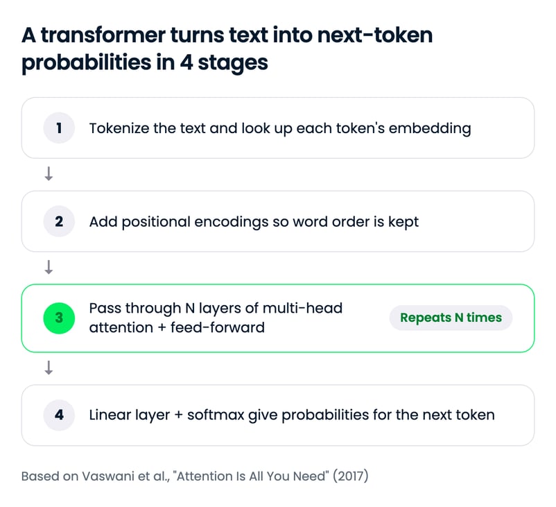
The architecture works in 4 stages. Text is split into tokens and mapped to embeddings, positional information is added, a stack of layers alternates multi-head self-attention with feed-forward networks (each wrapped in a residual connection and normalization), and a final linear layer with softmax turns the last vector into probabilities over the vocabulary. The original model paired an encoder with a decoder; most LLMs today keep only the decoder.
In this tutorial, I’ll walk through each stage of the original encoder-decoder design, then show how BERT, GPT, and today’s LLMs changed it. If you’d like the intuition first, read our explainers on the attention mechanism and self-attention.
TL;DR