TRIBE v2 Tutorial: Simulating Human Brain Activity from Video, Audio, and Text

What is TRIBE v2?

TRIBE v2 (TRImodal Brain Encoder) is a deep learning model that maps naturalistic stimuli onto predicted fMRI brain responses. Given a video clip, an audio file, or a block of text, the model outputs a predicted BOLD signal for each of the 20,484 vertices on the fsaverage5 cortical surface at 1 Hz, i.e., one prediction per second.

Predictions are for the average subject (not any specific person's brain), but the canonical group-average response that TRIBE v2 learned from 720 participants across four naturalistic datasets. The model's zero-shot predictions outperform single-subject fMRI recordings on the Human Connectome Project 7T dataset, which has the highest signal quality in the training set.

Key properties

The model is adapted from the paper called A foundation model of vision, audition, and language for in-silico neuroscience, which demonstrates that TRIBE v2 recovers the fusiform face area for faces, the parahippocampal place area for scenes, Broca's area for complex syntax, and the left-lateralized language network for speech without any fMRI data at inference time. 

TRIBE v2 Architecture Overview

TRIBE v2 has three stages that run in sequence for every inference call:

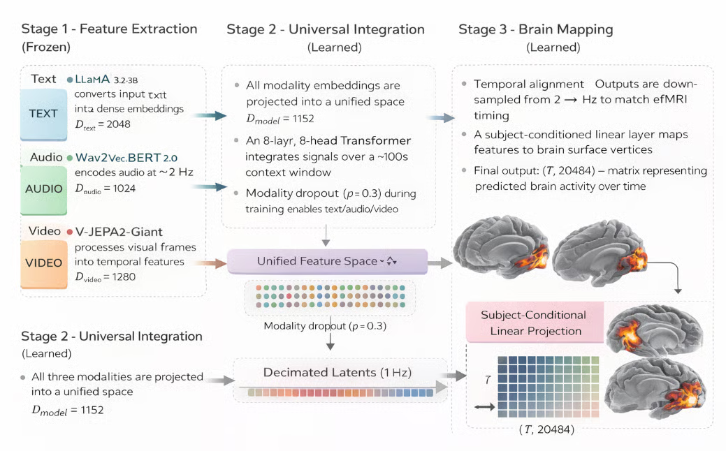
Figure: TRIBE v2 brain activity prediction model (Generated with AI)

Stage 1: Feature extraction (frozen)

Firstly, three separate pretrained encoders independently process each input modality into dense time-aligned embeddings. None of these encoders are updated during training (frozen), so TRIBE v2 inherits their representations as-is. Here are some metrics for feature extraction for each modality:

• Text: LLaMA 3.2-3B converts input text into dense embeddings (D = 2048)

• Audio: Wav2Vec-BERT 2.0 encodes audio signals at ~2 Hz (D = 1024)

• Video: V-JEPA2-Giant processes visual frames into temporal features (D = 1280)

Stage 2: Universal integration (learned)

The three embedding streams are fused into a single shared representation and processed by a Transformer that attends across time. This is where TRIBE v2's learned weights live and where cross-modal interactions are captured as follows:

• Shared representation: All modality embeddings are projected into a unified space (D_model = 1152)

• Transformer fusion: An 8-layer, 8-head Transformer integrates signals over a long (~100s) context window

• Modality flexibility: Modality dropout (p = 0.3) enables inference with any subset (text/audio/video)

Stage 3: Brain mapping (learned)

The fused latent representation is projected onto the cortical surface to produce the final fMRI prediction. This stage converts abstract model features into spatially and temporally resolved brain activity estimates. 

• Temporal alignment: Outputs are aligned and sampled at 1 Hz to match fMRI timing
• Cortical projection: A subject-conditioned linear layer maps features to brain surface vertices
• Final output: A matrix of (T, 20484) represents predicted brain activity over time

Since three feature extractors are frozen during training, the TRIBE v2 learns only the projection layers and transformer weights that integrate their outputs. This design choice is important because it means the model is robust to out-of-distribution stimuli, since it inherits the generalization of three large-scale pretrained models rather than being trained end-to-end on fMRI data alone.

Note: A key training trick is modality dropout. During training, each modality is independently zeroed out with probability 0.3. This forces the model to make meaningful predictions from any subset of modalities. So, at inference time, you can pass only audio or only text and still get a useful cortical prediction.

TRIBE v2 Demo: Predicting Brain Responses

In this section, we will build a step-by-step workflow that runs TRIBE v2 inference on text, audio, or video inputs and visualizes the predicted cortical activity as an interactive 3D brain heatmap. We will also run a comparison experiment that replicates the in-silico paradigm from the original paper. Finally, we’ll develop a Gradio app that anyone can use to explore the demo live.

Step 1: Prerequisites and hardware

Before starting, configure your Colab runtime. Note that you can also use any other service with a stable A100 GPU with high RAM.

• Open Runtime and select change runtime type
• Select A100 GPU and enable High RAM
• Click Save

TRIBE v2 loads three frozen encoders simultaneously, including LLaMA 3.2-3B (~7 GB), V-JEPA2-Giant (~14 GB), and Wav2Vec-BERT 2.0 (~1 GB), along with the TRIBE transformer weights. The total VRAM footprint is 28–32 GB. 

Note: A T4 (16 GB) will run out of memory when model.predict() loads LLaMA. Use the A100 (40 GB) or A100 with High RAM (80 GB) for better performance.

Verify your GPU before installing anything by running the following:

import subprocess, sys
result = subprocess.run(
    ['nvidia-smi', '--query-gpu=name,memory.total',
     '--format=csv,noheader,nounits'],
    capture_output=True, text=True)
print(result.stdout.strip())
import torch
assert torch.cuda.is_available(), "No GPU detected"
props = torch.cuda.get_device_properties(0)
assert props.total_memory > 30e9, (
    f"Need ≥40 GB VRAM. Got {props.total_memory/1e9:.0f} GB. Switch to A100.")
print(f"GPU: {props.name} — {props.total_memory/1e9:.0f} GB")

The subprocess.run() call invokes nvidia-smi with the --query-gpu flag to extract the GPU name and total VRAM. The two assert statements act as early exits; the first confirms CUDA is available, and the second verifies that total VRAM exceeds 30 GB. Failing loudly here is better than failing silently inside model.predict() 10 minutes later with a cryptic CUDA out-of-memory error.

Step 2: Fix the NumPy version conflict

Skip this step if you are not running this on a Google Colab. This is the first bug you will hit because Colab ships with NumPy 2.x by default. Several of TRIBE v2's internal dependencies, specifically neuralset, were compiled against NumPy <2.1, which removed the _center symbol from numpy._core.umath. The result is this error when you try to import tribev2:

ImportError
cannot import name '_center' from 'numpy._core.umath'
(/usr/local/lib/python3.12/dist-packages/numpy/_core/umath.py)

The fix is to pin NumPy to <2.1 before tribev2 or any of its dependencies are installed, then restart the runtime. Simply run the following cell, which uninstalls the current NumPy and replaces it with a version below 2.1. 

import subprocess, sys
print("Pinning NumPy to <2.1 (required for neuralset compatibility)...")
subprocess.run([sys.executable, '-m', 'pip', 'uninstall', '-y', 'numpy'])
subprocess.run([sys.executable, '-m', 'pip', 'install', '-q',
                'numpy>=1.26.4,<2.1.0'])

Once the environment and dependencies are finalized, we can proceed with installing TRIBE v2.

Step 3: Install TRIBE V2 

With the kernel freshly restarted and the pinned NumPy loaded, we can now safely install the tribev2 package from GitHub along with the visualization and UI libraries. 

import numpy as np
from packaging.version import Version
assert Version(np.__version__) < Version('2.1.0'), (
    f"NumPy is {np.__version__}. Run Step 2a and restart first.")
print(f"NumPy {np.__version__} Checked")
# Install tribev2 from GitHub 
!pip install -q 'tribev2[plotting] @ git+https://github.com/facebookresearch/tribev2.git'
!pip install -q 'gradio>=4.19.0' 'nilearn>=0.10.3' 'plotly>=5.18.0'

The tribev2[plotting] extra installs pyvista, a Python library for 3D visualization, and nilearn, a Python library for neuroimaging, alongside the core package. Installing from the GitHub URL directly ensures you get the latest commit without needing to clone the repository locally. 

The nilearn and gradio packages are installed separately because their version constraints are more flexible and benefit from being resolved independently of the tribev2 dependency graph.

Step 4: HuggingFace authentication

The text encoder uses LLaMA 3.2-3B, which is a gated model on HuggingFace. You need to explicitly accept Meta's license before the weights can be downloaded. Do this once:

• Visit HuggingFace and click Accept license
• Create a read token under Settings/Access Tokens 
• In Colab, click the key icon in the left sidebar and select Add secret. Finally, name your token “HF_TOKEN” and set “value: your token”.

Once your HF token is set, run the following code to log in to your account:

import os
# Load token from Colab Secrets
try:
    from google.colab import userdata
    os.environ['HF_TOKEN'] = userdata.get('HF_TOKEN')
    print("HF_TOKEN loaded from Colab Secrets")
except Exception:
    from huggingface_hub import login
    login()

The preferred path uses google.colab.userdata.get(), which reads from Colab's encrypted Secrets store, which cannot be accidentally exposed in a shared notebook link.

The fallback calls huggingface_hub.login(), which prompts interactively and masks the token as you type. Both paths write the token to os.environ['HF_TOKEN'], where the HuggingFace Hub library will automatically pick it up when downloading gated model weights.

Step 5: Load the pretrained model

With NumPy pinned, authentication configured, and LLaMA cached, we can now load the TRIBE v2 encoder checkpoint from HuggingFace. This downloads approximately 1 GB on the first run and takes a few seconds from cache on subsequent runs.

from pathlib import Path
from tribev2.demo_utils import TribeModel
import torch
CACHE_DIR = Path('/content/tribe_cache')
CACHE_DIR.mkdir(exist_ok=True)
print('Loading TRIBE v2 (first run downloads ~1 GB)...')
model = TribeModel.from_pretrained(
    'facebook/tribev2',
    cache_folder=str(CACHE_DIR)
)
print('Model loaded')
if torch.cuda.is_available():
    used  = torch.cuda.memory_allocated() / 1e9
    total = torch.cuda.get_device_properties(0).total_memory / 1e9
    print(f'VRAM after load: {used:.1f} / {total:.1f} GB')

TribeModel.from_pretrained() downloads the TRIBE encoder checkpoint from facebook/tribev2 on HuggingFace and saves it to cache_folder. This checkpoint contains the transformer integration weights and the subject block, but not the three feature extractors. Those are pulled separately when model.predict() first uses each modality.

After loading just the TRIBE encoder, roughly 2–4 GB of VRAM is allocated, while the remaining 24–28 GB will be consumed when model.predict() loads V-JEPA2-Giant and LLaMA 3.2-3B on first use.

Step 6: Fix the download timeout

After the TRIBE model loads, calling model.predict() on text input for the first time triggers a lazy download of the LLaMA 3.2-3B weights (~6 GB). HuggingFace Hub's default timeout is 10 seconds, producing this error mid-inference:

ReadTimeout
The read operation timed out
Computing word embeddings:  0%|  | 0/9 [00:10<?, ?it/s]

To fix this, raise the timeout environment variables, then pre-download LLaMA explicitly using snapshot_download so you get visible progress and automatic resume on interruption rather than a silent failure buried inside predict().

import os
os.environ['HF_HUB_DOWNLOAD_TIMEOUT'] = '300'   
os.environ['HF_HUB_HTTP_TIMEOUT']     = '300' 
from huggingface_hub import snapshot_download
print("Pre-downloading LLaMA 3.2-3B (~6 GB)...")
print("Runs once — subsequent calls load from cache.\n")
snapshot_download(
    repo_id        = "meta-llama/Llama-3.2-3B",
    cache_dir      = "/content/tribe_cache/llama",
    ignore_patterns= ["*.bin"], 
)
print("\n LLaMA 3.2-3B cached")

snapshot_download() downloads an entire repository to the local cache using HuggingFace's range-request protocol, which means it resumes automatically if the connection drops mid-file. The ignore_patterns=["*.bin"] argument skips the older PyTorch binary format and downloads only the safetensors files, reducing total download size by roughly 40%.

Step 7: Brain visualization helpers

Before running real inference, we set up the visualization layer. These helper functions convert the raw (T, 20484) prediction array into interactive 3D brain heatmaps using nilearn. 

TRIBE v2 returns predictions as a NumPy array of shape (T, 20484), where T is the number of seconds of input. The first 10,242 vertices are in the left hemisphere, and the remaining 10,242 are in the right hemisphere. 

We use nilearn.plotting.view_surf to render each hemisphere as an interactive WebGL surface. The inflated mesh exposes sulcal geometry that would otherwise be hidden in the folds, and the sulcal depth map provides anatomical reference under the heatmap.

Step 7.1: Download the fsaverage5 mesh

The fsaverage5 mesh is the standard FreeSurfer cortical template that TRIBE v2 uses as its output space. We download it once here so all subsequent visualization calls can reference it without re-fetching from the network.

import numpy as np
from nilearn import datasets as nl_datasets
from nilearn.plotting import view_surf
from IPython.display import display, HTML
N_PER_HEMI = 10242   # fsaverage5: 10242 vertices per hemisphere
print('Fetching fsaverage5 mesh...')
fsavg = nl_datasets.fetch_surf_fsaverage(mesh='fsaverage5')
print('Mesh ready')
print('Keys:', [k for k in fsavg.keys() if k != 'description'])

The fetch_surf_fsaverage(mesh='fsaverage5') downloads the FreeSurfer fsaverage5 template from nilearn's CDN and caches it. It also returns a Bunch object (dictionary) with keys like infl_left, infl_right, sulc_left, and sulc_right. 

Step 7.2: Split hemispheres and render

This sub-step defines the three core functions that all visualization in this tutorial depends on. split_hemis() function partitions the vertex array, render_hemi() function builds the interactive WebGL surface for one hemisphere, and show_brain() function assembles both into the side-by-side layout.

def split_hemis(v):
    n = v.shape[0]
    if n == 2 * N_PER_HEMI:
        return v[:N_PER_HEMI], v[N_PER_HEMI:]
    return v[:n//2], v[n//2:]  
def render_hemi(pred_vec, hemi='left', title=''):
    lh, rh = split_hemis(pred_vec)
    data = lh if hemi == 'left' else rh
    vmax = max(float(np.percentile(np.abs(data), 99)), 1e-6)
    return view_surf(
        surf_mesh = fsavg[f'infl_{hemi}'],   
        surf_map  = data,
        bg_map    = fsavg[f'sulc_{hemi}'],   
        hemi      = hemi,
        threshold = '20%',  
        cmap      = 'hot',    
        black_bg  = True,
        vmax      = vmax,
        bg_on_data= True,     
        colorbar  = True,
        title     = title,
    )
def show_brain(pred_vec, title='', t=None):
    sfx = f' — t={t}s' if t is not None else ''
    lv  = render_hemi(pred_vec, 'left',  f'{title} [Left]{sfx}')
    rv  = render_hemi(pred_vec, 'right', f'{title} [Right]{sfx}')
    html = (
        '<div style="display:flex;gap:10px;background:#000;'
        'border-radius:10px;">'
        f'<div style="flex:1">{lv.get_iframe(width="100%",height="460px")}</div>'
        f'<div style="flex:1">{rv.get_iframe(width="100%",height="460px")}</div>'
        '</div>'
    )
    display(HTML(html))

Let’s understand the function of each helper function in detail:

• The split_hemis() function slices the prediction vector at index 10,242, which is the standard split point for the fsaverage5 mesh in FreeSurfer's convention. The left hemisphere occupies indices 0–10241 and the right hemisphere occupies 10242–20483. The fallback branch at the bottom handles edge cases where the model returns a non-standard vertex count.

• Inside the render_hemi() function, the vmax is computed as the 99th percentile of absolute activation values rather than the true maximum. This prevents a single extreme vertex from collapsing the entire colormap into a narrow range, making the spatial pattern visible. 

• The view_surf() function returns a SurfaceView object containing 2.4 MB of self-contained WebGL HTML. The get_iframe() call wraps this in an <iframe> tag sized to the given dimensions. So, when we call display(HTML(...)) with two iframes side by side, it produces the split left/right hemisphere layout.

With the model loaded and visualization helpers ready, we can run our first real inference. 

Step 8: Run inference

TRIBE v2's inference is a two-step process. First, model.get_events_dataframe() extracts time-aligned events from the input, along with word timings from text, Wav2Vec embeddings at 2 Hz from audio, or V-JEPA2 embeddings at 2 Hz from video frames. 

The resulting events DataFrame is then passed to model.predict(), which runs the transformer and subject block to produce the final cortical predictions.

import tempfile, os
SAMPLE_TEXT = '''
The brain processes language through a distributed network in the left hemisphere.
Broca's area coordinates syntactic structure, while Wernicke's area handles semantics.
Together they form the language circuit activated when reading or hearing speech.
'''
tmp = tempfile.NamedTemporaryFile(delete=False, suffix='.txt', mode='w')
try:
    tmp.write(SAMPLE_TEXT.strip())
    tmp.flush()
    os.fsync(tmp.fileno())   
    tmp.close()
    events = model.get_events_dataframe(text_path=tmp.name)
finally:
    if os.path.exists(tmp.name):
        os.unlink(tmp.name) 
print(f'Events: {events.shape}')
print(events[['type', 'start', 'duration']].head(8))
print('\nRunning model.predict()...')
preds, segments = model.predict(events=events)
preds = np.asarray(preds)
print(f'Prediction shape: {preds.shape}')
print(f'  T = {preds.shape[0]}s   (1 Hz fMRI frequency)')
print(f'  V = {preds.shape[1]} vertices  (fsaverage5 cortical surface)')

The write sequence of tmp.write(), tmp.flush(), os.fsync(tmp.fileno()), tmp.close() is the critical fix for a subtle bug. If you call get_events_dataframe() inside a with block before the file is closed, Python's internal write buffer may not yet have been synced to the OS, and tribev2 will read an empty file and raise ValueError. The os.fsync() call guarantees the OS page cache is flushed to disk before tribev2 opens the path.

The model.predict() returns a tuple of (preds, segments). The preds array has shape (T, 20484), one cortical prediction per second of input across all 20,484 fsaverage5 vertices. Wrapping it in np.asarray() ensures it is a plain NumPy array regardless of what internal type the model returns. Once you have preds, you can visualize the cortical response at any timestep:

T = preds.shape[0]
print(f'Timesteps: 0 to {T-1}')
T_SHOW = min(5, T - 1)
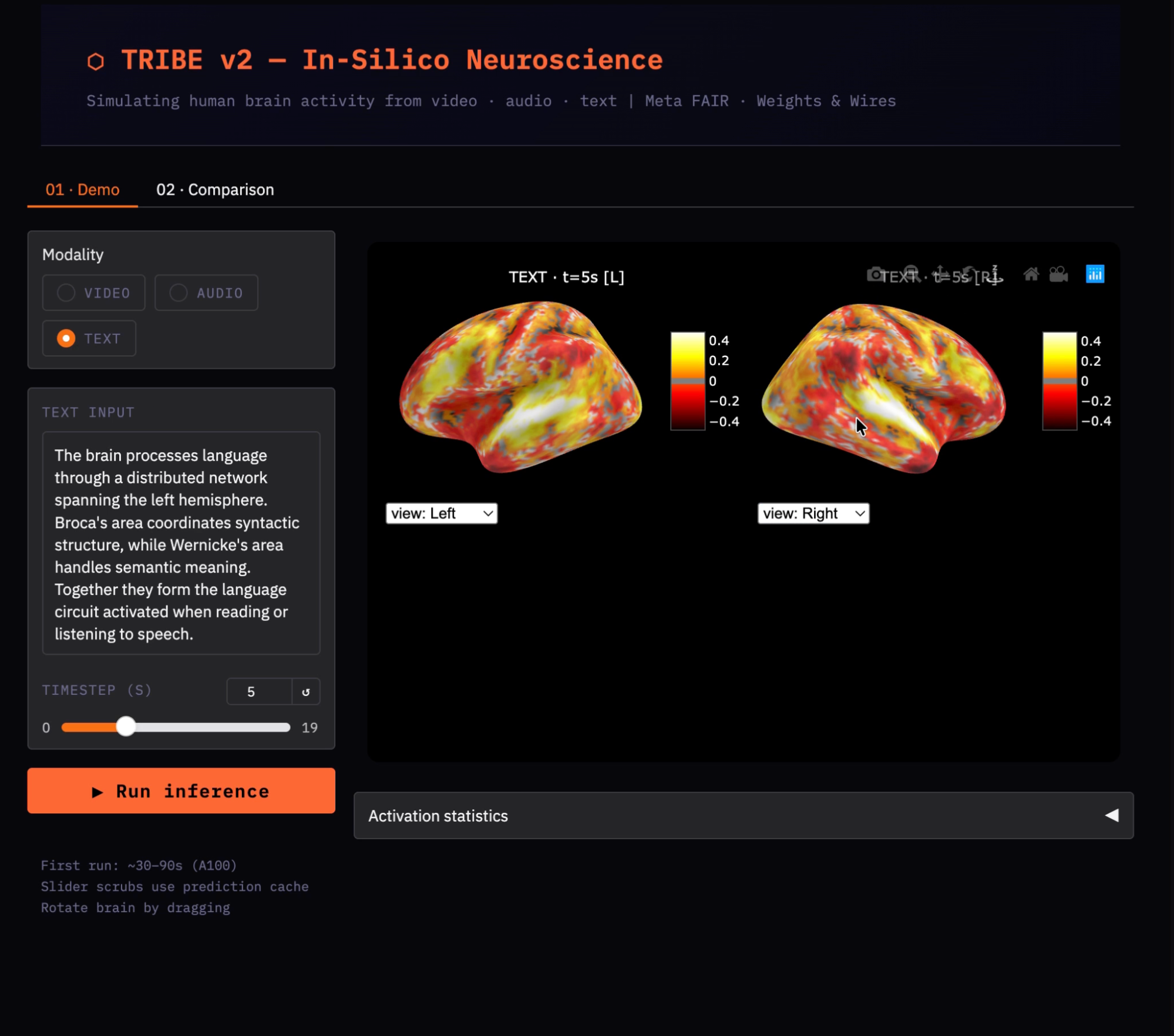
show_brain(preds[T_SHOW], title='Language stimulus', t=T_SHOW)

We default to t=5 because the BOLD (Blood-Oxygen-Level-Dependent) signal has a hemodynamic delay, and the vascular response to neural activity peaks approximately 5–6 seconds after stimulus onset. Visualizing at t=0 shows near-zero activation regardless of the stimulus content, since the brain's vascular response has not yet built up. The min(5, T-1) guard prevents an index error when the input produces fewer than 6 timesteps.

Step 9: Comparison experiment

A single activation map tells you which areas are active, but it does not tell you what makes one stimulus different from another. This step runs two inputs through the model and computes a contrast map (A − B) to isolate the region-specific differences between language content and visual/spatial content.

Step 9.1: Define a reusable inference helper

Rather than repeating the write -> flush -> close -> infer pattern for each condition, we wrap it in a single text_to_preds() function. This ensures the critical file-flushing steps are never accidentally omitted for either condition.

TEXT_A = '''
She spoke slowly and clearly, her voice filling the quiet room.
Every sentence carried meaning, and each word was chosen with care.
Language connects us, the professor said, bridging minds across time.
'''
TEXT_B = '''
The canyon walls rose steeply, layers of red and orange sandstone.
A hawk circled overhead, its wings barely moving in the thermal current.
Shadows shifted as the sun tracked its arc across the open desert sky.
'''
def text_to_preds(text):
    tmp = tempfile.NamedTemporaryFile(
        delete=False, suffix='.txt', mode='w', encoding='utf-8')
    try:
        tmp.write(text.strip())
        tmp.flush()
        os.fsync(tmp.fileno())
        tmp.close()
        evts = model.get_events_dataframe(text_path=tmp.name)
        p, _ = model.predict(events=evts)
        return np.asarray(p)
    finally:
        if os.path.exists(tmp.name):
            os.unlink(tmp.name)
print('Condition A: language content...')
preds_a = text_to_preds(TEXT_A)
print('Condition B: visual/spatial content...')
preds_b = text_to_preds(TEXT_B)

We use two text passages with distinct semantic content, with the expected finding that language content drives the left-hemisphere temporal cortex more, while visual/spatial content recruits the occipital and posterior parietal cortex more.

The text_to_preds() function encapsulates the full pipeline into a single reusable function, applying the same safe pattern from Step 8 so the temp file is always fully flushed before tribev2 reads it. The encoding='utf-8' argument is explicit to avoid platform-dependent encoding issues.

Step 9.2: Render raw activations and contrast map

Now that both conditions are predicted, we visualize each one individually and then subtract them vertex-by-vertex to produce the contrast map. 

T_shared = min(preds_a.shape[0], preds_b.shape[0])
t_show   = min(5, T_shared - 1)
print('\n[A] Language content:')
show_brain(preds_a[t_show], title='Condition A: Language', t=t_show)
print('\n[B] Visual/spatial content:')
show_brain(preds_b[t_show], title='Condition B: Visual', t=t_show)
print('\n[A − B] Contrast: Language > Visual')
show_brain(preds_a[t_show] - preds_b[t_show], title='Contrast A − B', t=t_show)

The contrast map preds_a[t_show] - preds_b[t_show] is a direct vertex-wise subtraction where positive values indicate regions where condition A activates more, and negative values indicate regions where condition B activates more. 

Since both conditions share the same text-processing pathway, the raw maps will look broadly similar. This contrast map highlights domain-specific differences between language and visual content.

Step 9.3: Plot the temporal difference

The brain heatmaps show spatial patterns at a single moment in time. This step adds a temporal perspective, such as how does overall activation compare between conditions across all timesteps, and when do the two conditions diverge most strongly? 

import matplotlib.pyplot as plt
diff_norms = [
    np.linalg.norm(preds_a[i] - preds_b[i])
    for i in range(T_shared)
]
fig, (ax1, ax2) = plt.subplots(1, 2, figsize=(14, 3.5))
ax1.plot(np.abs(preds_a).mean(axis=1)[:T_shared],
         color='#e74c3c', linewidth=2, label='A: Language')
ax1.plot(np.abs(preds_b).mean(axis=1)[:T_shared],
         color='#3498db', linewidth=2, label='B: Visual')
ax1.set_title('Mean cortical activation over time')
ax1.set_xlabel('Time (s)'); ax1.legend(); ax1.grid(True, alpha=0.3)
ax2.plot(diff_norms, color='#f39c12', linewidth=2)
ax2.fill_between(range(T_shared), diff_norms, alpha=0.2, color='#f39c12')
ax2.set_title('||A − B|| difference over time')
ax2.set_xlabel('Time (s)'); ax2.grid(True, alpha=0.3)
plt.tight_layout(); plt.show()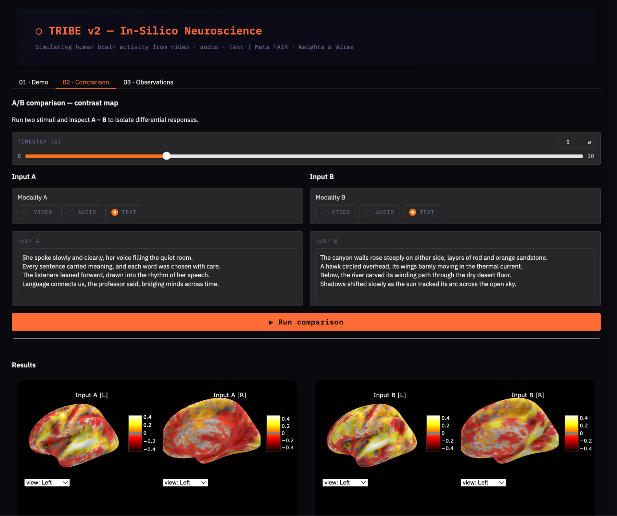

The left plot tracks np.abs(preds).mean(axis=1), which is the mean absolute activation collapsed across all 20,484 vertices at each second. This shows how strongly each condition engages the cortex and when the response peaks. Taking the absolute value is important because predicted BOLD values can be negative (deactivation), and we want the magnitude rather than the signed mean.

The right plot tracks the L2 norm of the difference vector at each timestep, np.linalg.norm(preds_a[i] - preds_b[i]). A peak in this curve around t=5–7s is consistent with the hemodynamic delay so, both conditions need time for the BOLD response to build before they diverge. The fill_between() shading makes the onset and peak of divergence visually clear.

Step 10: Launch the Gradio demo

This final step wraps the inference and visualization logic in a Gradio app with a clean UI, a timestep slider, and an A/B comparison tab. 

import gradio as gr
_pred_cache = {}   
def _infer(mod, vid, aud, txt):
    """Run inference and cache the result. Subsequent calls return cached array."""
    key = (mod, vid, aud, hash(txt or ''))
    if key not in _pred_cache:
        if mod == 'video':
            evts = model.get_events_dataframe(video_path=vid)
        elif mod == 'audio':
            evts = model.get_events_dataframe(audio_path=aud)
        else:
            tmp = tempfile.NamedTemporaryFile(delete=False, suffix='.txt', mode='w')
            tmp.write((txt or '').strip()); tmp.flush()
            os.fsync(tmp.fileno()); tmp.close()
            evts = model.get_events_dataframe(text_path=tmp.name)
            os.unlink(tmp.name)
        p, _ = model.predict(events=evts)
        _pred_cache[key] = np.asarray(p)
    return _pred_cache[key]
demo.launch(
    share      = True,    
    debug      = False,
    server_name= "0.0.0.0",
)

Here is how the Gradio UI and inference pipeline come together:

• The _infer() function acts as the central inference layer, handling all three modalities (video, audio, and text) by preparing inputs, calling model.predict(), and returning the predicted brain activity.

• A prediction cache is used to store results based on a key composed of the modality, input paths, and a hash of the text. This ensures that identical inputs do not trigger repeated model inference.

• The caching mechanism is critical because UI components like sliders trigger callbacks frequently. Without caching, each interaction would re-run inference (taking up to ~60 seconds), whereas with caching, results are returned instantly after the first run.

• The interface provides two tabs, one with a single-input mode with a timestep slider to explore brain activity over time, and a comparison mode that runs two inputs and visualizes their difference as a contrast heatmap.

Finally, demo.launch() is configured with share=True to generate a public URL and server_name="0.0.0.0" to allow external access, making the app easily deployable.

Observations and Practical Insights on TRIBE v2

After running the demo across different inputs (video, audio, and text), a few consistent patterns emerge that help interpret TRIBE v2’s outputs. Some insights from the demo are:

• Temporal dynamics: As the input progresses, the brain activity changes over time rather than staying static. You’ll notice that activation gradually builds and shifts across regions, especially within the first few seconds. This reflects the delayed nature of the underlying signal and confirms that the model is capturing time-dependent responses.
• Effect of visual inputs on posterior regions: In the video-based examples, the strongest activations appear toward the back of the brain. This aligns with visual processing regions, indicating that the model is responding appropriately to visual stimuli.
• Contrast maps: When comparing two inputs, the difference heatmap is often more informative than individual maps. Instead of broad activation everywhere, the contrast highlights where the brain responds differently to each stimulus, making it easier to interpret the effect of different modalities.

Common pitfalls

The model does not claim to be 100% accurate, and comes with its own pitfalls:

• Noisy maps: It is observed that very short inputs (a few seconds) often produce diffuse, low-intensity activations that are hard to interpret. Inputs must be a certain length (15–30 seconds) to provide enough context for the model to generate meaningful patterns.
• Missing modalities: If you run audio or text without video, you may see warnings about certain extractors being removed. This is expected as the model simply disables unused branches and continues with available inputs.
• Caching: Without caching, every UI interaction (like moving the slider) would trigger a full model run, making the demo unusable. With caching enabled, predictions are computed once and reused, allowing smooth, real-time exploration.
• Environment inconsistencies: Any changes in dependencies (especially NumPy versions) or improper file handling (like unflushed text files) can lead to silent failures.

Limitations

TRIBE v2 is a powerful research tool, but it has important constraints that affect how its outputs should be interpreted. Understanding these limits is essential before drawing any scientific or clinical conclusions from the predictions.

• Average subject: Predictions represent the population means. Individual brains differ in cortical anatomy, functional organization, and noise profile. Fine-tuning on ~1 hour of individual fMRI data is supported by the model, but beyond this tutorial's scope.
• fMRI resolution: The BOLD signal has ~1 Hz temporal resolution and ~4 mm spatial resolution. TRIBE v2 inherits both limits but cannot capture millisecond neural dynamics or sub-gyral spatial detail.
• Passive observer: The model predicts responses to stimuli presented to a passive observer. It has no representation of attention, motor output, social interaction, or any active cognitive state.
• Modality scope: Only vision, audition, and language are modeled. However, modalities such as olfaction, touch, proprioception, and pain are absent.
• Not a clinical tool: Predictions should not be used for diagnosis, treatment planning, or any clinical application.

Conclusion

In this tutorial, we built a working TRIBE v2 pipeline on Google Colab A100: from resolving two concrete bugs (the NumPy 2.x version conflict and the HuggingFace download timeout) through running real cortical predictions, to visualizing them as interactive 3D brain heatmaps and running a comparison experiment that replicates the paper's in-silico paradigm.

The four most important engineering lessons from this tutorial are: 

1. Pin NumPy to <2.1 and restart the runtime before installing tribev2

2. Set HF_HUB_DOWNLOAD_TIMEOUT=300 and pre-download LLaMA with snapshot_download before calling model.predict()

3. Always write → flush() → fsync() → close() temp files before passing their path to the model

4. Cache predictions in a dictionary, so UI slider interactions never re-run inference.

From here, two natural extensions stand out. The first is richer stimuli: real movie clips or podcast segments spanning 30–60 seconds produce much clearer temporal dynamics and spatial patterns than short text passages. 

The second is individual fine-tuning: given ~1 hour of fMRI data from a specific subject, TRIBE v2's subject block can be fine-tuned in one epoch to produce personalized predictions that outperform the group-average model by 2–4x according to the paper's results.

The full notebook is available on the TRIBE v2 GitHub repository. The paper is worth reading in full, particularly Section 2.5 (in-silico vision experiments) and Section 2.8 (multimodal integration insights), which show what this kind of tooling makes possible for neuroscience research.