Likelihood Ratio: An Important Measure of Statistical Evidence

Have you seen the term "likelihood ratio" in a regression output or a study and had no idea what it's telling you?

You're not the only one. The term is often seen in hypothesis testing, model comparison, classification, and diagnostic testing, and each field uses it a bit differently. Most explanations also start with a test statistic and a chi-square distribution before you even know what a likelihood is. So you end up with a number you can compute but can't explain.

In short, likelihood shows how well a parameter value or a statistical model explains the data you've observed. A likelihood ratio divides one likelihood by another, so you can see which of two hypotheses gets more support from the data, and by how much.

In this article, I'll walk you through the core idea and the formula, the likelihood ratio test and how to interpret it, and where you'll see likelihood ratios in practice.

Need a statistics refresher? Browse our catalog of Probability and Statistics courses and find the perfect fit.

What Is a Likelihood Ratio?

A likelihood ratio is the likelihood of the observed data under one hypothesis divided by the likelihood of the same data under another hypothesis. The two hypotheses can be two parameter values or two full statistical models.

The question it answers is which explanation accounts for the data better, not whether the data are likely.

That's an important difference. Any specific sequence of 20 coin flips has a probability of about one in a million under a fair coin, so a small likelihood on its own doesn't tell you much. It only makes sense next to another likelihood.

Let's say you flip a coin 10 times and get 8 heads. One hypothesis says the coin is fair, with a 0.5 probability of heads. Another says it's biased, with a 0.8 probability of heads.

Both hypotheses can produce 8 heads, but the biased coin produces that result much more often. So the data give more support to the second hypothesis, and the likelihood ratio puts a number on how much more. I'll calculate the exact values in the example section later in this article.

Likelihood and probability use the same formula, but they answer different questions:

• Probability: Fixes the parameter and asks how probable different outcomes are - for example, the chance of 8 heads in 10 flips with a fair coin
• Likelihood: Fixes the observed data and asks how well different parameter values explain them - for example, how well a 0.5 versus a 0.8 probability of heads explains 8 heads in 10 flips

Probabilities across all possible outcomes add up to 1, but likelihoods across all possible parameter values don't. That's why a likelihood isn't the probability that a hypothesis is true, and neither is a likelihood ratio.

How Does a Likelihood Ratio Work?

Every likelihood ratio follows the same five steps:

1. Observe the data: Collect the sample you want to explain, like 8 heads in 10 flips
2. Calculate the first likelihood: Find how probable the observed data are under hypothesis A
3. Calculate the second likelihood: Do the same under hypothesis B
4. Divide: Put one likelihood in the numerator and the other in the denominator
5. Interpret the ratio: Check which hypothesis the data support more, and by how much

The meaning of the ratio depends on which likelihood goes on top. With hypothesis A in the numerator:

• Ratio above 1: The data are more probable under A, so A gets more support
• Ratio below 1: The data are more probable under B, so B gets more support
• Ratio equal to 1: Both hypotheses explain the data equally well, and the data don't favor either one

A ratio of 4 means the observed data are four times as probable under A as under B. It doesn't mean A is four times as likely to be true.

If you swap the numerator and denominator, you'll get the reciprocal. A ratio of 4 in favor of A becomes 0.25, which says the same thing from the side of B.

Conventions differ between fields. The likelihood ratio test usually puts the null hypothesis in the numerator, so small values count as evidence against it, while many other applications put the alternative hypothesis on top.

So before you interpret any likelihood ratio, check which hypothesis is in the numerator.

Likelihood Ratio Formula

The basic likelihood ratio divides one likelihood of the data by another:

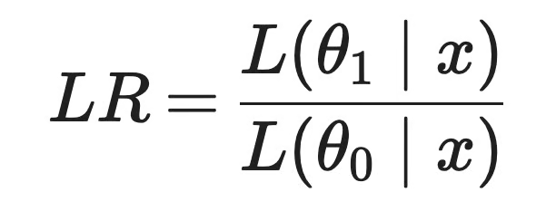
Likelihood ratio formula

Here's what each term means:

• x: The observed data, like 8 heads in 10 flips
• theta_1 and theta_0: The two parameter values or hypotheses you want to compare, like a 0.8 and a 0.5 probability of heads
• L(theta | x): The likelihood of theta given the data, which equals the probability of x when theta is the true parameter, or its density for continuous data

With independent observations, the likelihood is a product of one probability per observation:

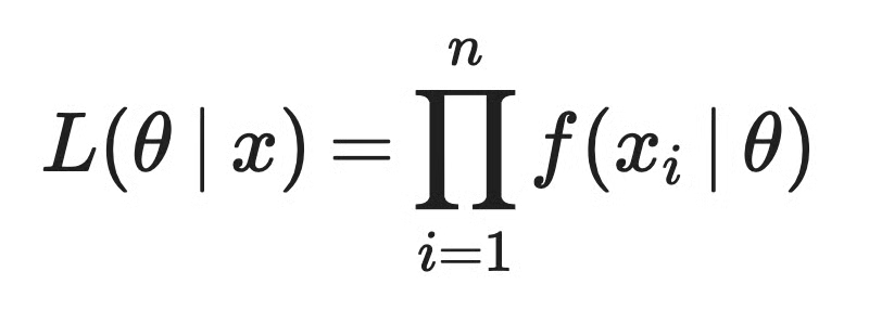
Likelihood with independent observations

And that's where the problems begin. Each factor is below 1, so the product reduces fast as the sample grows.

The probability of a specific sequence of 1,000 flips under a fair coin is about 9.3 * 10^-302, which is close to the smallest number a 64-bit float can store. At 2,000 flips, 0.5 ** 2000 in Python returns 0.0.

Logarithms are a way to get around. The log of a product is the sum of the logs, so the log-likelihood turns a product of tiny numbers into a sum of manageable ones:

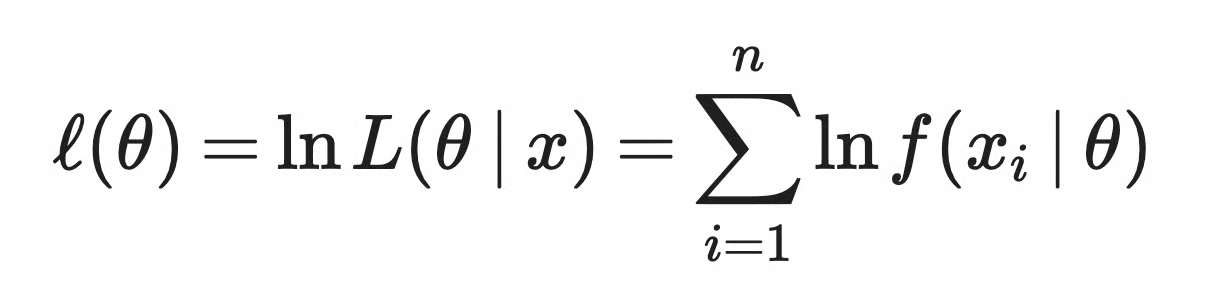
Log likelihood

The ratio becomes a difference:

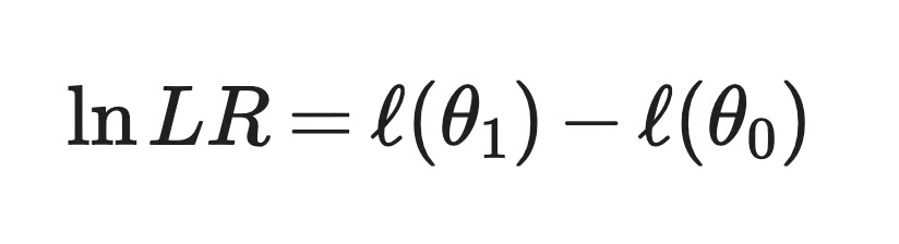
Log likelihood ratio

Sums are also simpler to differentiate than products, which is why maximum likelihood estimation works with log-likelihoods too.

The log version reads the same way as the ratio, just around 0 instead of 1. A value of 0 means equal support, positive values favor theta_1, and negative values favor theta_0.

Likelihood Ratio Example

Let's go back to the coin from earlier. You flip it 10 times and get 8 heads and 2 tails.

The two hypotheses are:

• Hypothesis 0: The coin is fair, so p = 0.5

• Hypothesis 1: The coin is biased toward heads, so p = 0.8

The number of heads in 10 flips follows a binomial distribution, so the likelihood of each hypothesis is:

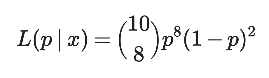
Likelihood ratio example

Under the fair coin hypothesis:

Likelihood ratio example

Under the biased coin hypothesis:

Likelihood ratio example

The likelihood ratio is:

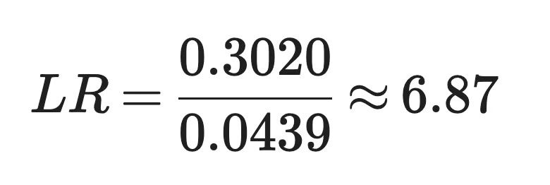
Likelihood ratio example

The binomial coefficient of 45 appears in both likelihoods, so it cancels out in the ratio. You'd get the same 6.87 from the probability of the exact sequence of flips.

In plain English, the observed data are about 6.9 times as probable if the coin lands heads 80% of the time than if it's fair. That's it.

The ratio doesn't say the coin is 6.9 times as likely to be biased. To get a probability that either hypothesis is true, you need prior probabilities for both. With 50/50 prior odds, the posterior odds would be 6.87 to 1, or about 87% for the biased coin, but that number depends on the prior you chose.

The support is also relative to these two hypotheses only. A value like p = 0.7 wasn't part of the comparison. Here, 0.8 also happens to be the maximum likelihood estimate, because 8 out of 10 flips came up heads, so no other value of p gets more support from this data.

What Is a Likelihood Ratio Test?

The coin example compared two fixed values of p. Most questions in statistics are broader, like whether a couple of extra predictors improve a regression model.

The likelihood ratio test answers that kind of question. It compares two nested models, which means the smaller model is a special case of the larger one:

• Restricted model: Represents the null hypothesis, with some parameters fixed, usually at 0
• Full model: Represents the alternative hypothesis, with those parameters free to take any value

The test has five steps:

1. Fit the restricted model: Find the parameter values that maximize its likelihood
2. Fit the full model: Do the same with the extra parameters included
3. Compare the maximized likelihoods: Take their ratio, or the difference of their log-likelihoods
4. Calculate the test statistic: Turn that comparison into a number with a known distribution
5. Get the p-value: Check how extreme the statistic is if the null hypothesis is true

Each model is evaluated at its maximum likelihood estimate, not at a parameter value you chose in advance. That's the main difference from the coin example.

The likelihood ratio compares any two hypotheses and gives you relative support, but no p-value and no decision. The LRT takes a ratio of maximized likelihoods from nested models, converts it into a test statistic, and uses its distribution to decide whether to reject the null hypothesis. Every LRT uses a likelihood ratio, but not every likelihood ratio is part of an LRT - the diagnostic likelihood ratios later in this article are one example.

Likelihood Ratio Test Statistic

The LRT starts with the ratio of maximized likelihoods, with the restricted model on top:

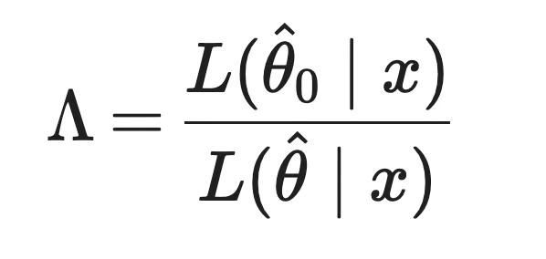
Likelihood ratio test statistic

Here, theta_hat_0 is the maximum likelihood estimate under the restricted model, and theta_hat is the estimate under the full model. The full model contains the restricted one, so it always fits at least as well. This means lambda is between 0 and 1.

The test statistic is:

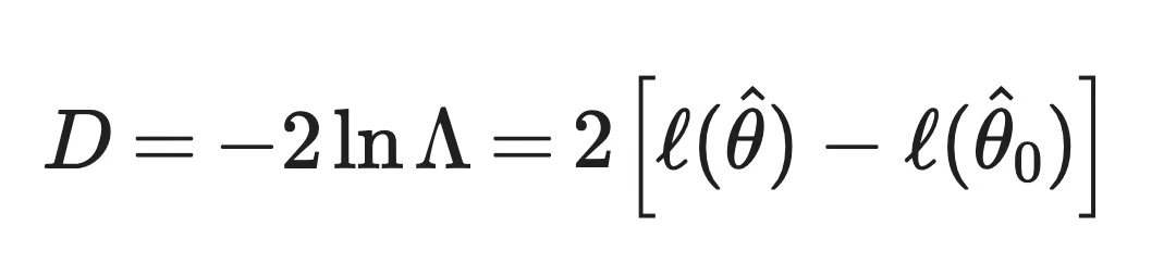
Likelihood ratio test statistic

Logarithms are there for the same reason as before. They turn a ratio of tiny numbers into a difference of log-likelihoods, which every statistical package reports.

The -2 has two jobs. Since lambda <= 1, ln(lambda) is 0 or negative, so the minus sign turns it into a positive number that grows as the full model fits better. The factor of 2 scales the statistic so it follows a chi-square distribution. For generalized linear models, D is the same as the difference in deviance between the two models, which is why you'll often see it reported that way.

Wilks' theorem makes the test work. It says that when the null hypothesis is true and standard regularity conditions hold, D approximately follows a chi-square distribution as the sample size grows. In plain terms, the models need to be nested, and the null parameter values can't be on the edge of the allowed parameter range. The limitations section later in this article covers what happens when these conditions break.

The degrees of freedom usually equal the difference in the number of free parameters between the two models. If the full model adds two predictors, you compare D to a chi-square distribution with 2 degrees of freedom.

So the same reference distribution works for logistic regression, Poisson regression, and most other models fit by maximum likelihood.

How to Interpret a Likelihood Ratio Test

Let's say you want to predict whether a customer cancels a subscription. The dataset has 1,000 customers, and about 32% of them churned.

You fit two logistic regression models:

• Restricted model: Predicts churn from tenure_months only, with a log-likelihood of -556.88

• Full model: Adds monthly_charges and support_tickets, with a log-likelihood of -515.99

Here's how each part of the test applies to this example:

• Null hypothesis: The coefficients of monthly_charges and support_tickets are both 0, so the extra predictors don't improve the fit

• Alternative hypothesis: At least one of those two coefficients isn't 0

• Test statistic: D = 2 * (-515.99 - (-556.88)) = 81.78

• Degrees of freedom: The full model has two more parameters, so the test uses 2 degrees of freedom

• P-value: The probability of a statistic this large or larger under a chi-square distribution with 2 degrees of freedom, which is about 1.7 * 10^-18

That p-value is far below any common threshold, like 0.05. You reject the null hypothesis and conclude that the data give strong evidence that the extra predictors improve the fit.

But rejecting the null doesn't mean the full model is the better choice for your use case.

With large samples, even tiny improvements in fit produce small p-values. The test doesn't tell you how big the effects are or how well the model predicts new data. Check the coefficients and the performance on held-out data before you keep the larger model.

And a large p-value doesn't prove the extra predictors are useless. It only means the data don't give enough evidence against the null hypothesis.

An LRT tells you whether extra parameters improve the fit, and deciding whether that improvement matters is still your job.

Likelihood Ratio Tests for Regression Models

You'll see the LRT most often when you compare regression models. The idea always stays the same - fit a restricted model, fit a full model, and compare their maximized log-likelihoods.

Logistic regression

Logistic regression is the most common place to see the LRT.

The interpretation section compared a model with tenure_months to a model that also has monthly_charges and support_tickets. You can go one step further and compare the full model to an intercept-only model, which predicts the same churn probability for every customer.

On the same churn data, the intercept-only model has a log-likelihood of -627.62, and the full model has -515.99. This gives D = 2 * (-515.99 - (-627.62)) = 223.27 with 3 degrees of freedom, one for each predictor, and a p-value of about 3.9 x 10^-48.

This test asks whether the predictors, taken together, explain churn better than no predictors at all. It's the logistic regression version of the overall F-test in linear regression, and statsmodels reports it in the model summary as LLR p-value.

Generalized linear models

Logistic regression is one member of a larger family called generalized linear models, or GLMs. The family also includes Poisson regression for counts and gamma regression for positive continuous outcomes, among others.

Every GLM reports a deviance, which measures how far the model is from a perfect fit. For two nested GLMs, the difference in their deviances equals the LRT statistic D, so the test is often called an analysis of deviance.

The degrees of freedom work the same way as before, as the difference in the number of parameters. For models with an estimated dispersion parameter, like gamma or Gaussian GLMs, an F-test on the deviance difference is often used instead of the chi-square version.

Other likelihood-based models

Any model fit by maximum likelihood can use an LRT, as long as the models are nested. For example:

• Mixed-effects models: Compare models with and without a fixed effect, fit with maximum likelihood rather than REML
• Survival models: Test whether a covariate improves a Cox proportional hazards model, which uses a partial likelihood
• Time series models: Compare ARIMA models of different orders
• Genetics: Test for linkage between genes, where LOD scores are base-10 log likelihood ratios

Likelihood Ratio vs. Related Statistical Tests

The LRT is similar to the Wald test and the score test. All three test the same null hypothesis, and all three follow a chi-square distribution in large samples. The difference is in which models you fit and what you measure.

Likelihood ratio test vs. Wald test

The LRT fits both models and compares their log-likelihoods. The Wald test fits only the full model and checks how far each estimate is from its null value, measured in standard errors.

For a single coefficient, the Wald statistic is the estimate divided by its standard error. The p-values in a regression summary table usually come from this test.

The Wald test is fast, since you only fit one model. But it depends on how you parametrize the model, and in logistic regression it can behave poorly when coefficients are very large, because the standard error grows faster than the estimate. The LRT doesn't have either problem, so it's the safer choice.

Likelihood ratio test vs. score test

The score test fits only the restricted model.

It looks at the slope of the log-likelihood at the null parameter values. If the null hypothesis is right, the slope should be close to 0. A steep slope means the likelihood would increase if you let those parameters move away from the null.

This makes the score test handy when the full model is expensive or hard to fit. It's also known as the Lagrange multiplier test, and it's often used to screen candidate predictors before you add them.

Likelihood ratio test vs. chi-square test

The LRT statistic follows a chi-square distribution in large samples, but that doesn't make the LRT a "chi-square test" in the usual sense.

"Chi-square test" is a broad label for any test whose statistic follows a chi-square distribution. Most of the time, people use it to mean Pearson's chi-square test for independence or goodness of fit in contingency tables.

The two are connected, though. The likelihood ratio version of Pearson's test is called the G-test, and it compares observed and expected counts with log-likelihoods instead of squared differences. In large samples, both give similar results.

Here's how the three model-based tests compare:

Likelihood ratio compared to other statistical tests

Likelihood Ratio vs Odds Ratio

Both terms have "ratio" in the name, and both are common in logistic regression. That's where the similarity ends.

A likelihood ratio compares how well two hypotheses explain the observed data. An odds ratio compares the odds of an outcome between two groups or conditions.

Odds are the probability of an event divided by the probability that it doesn't happen. A 25% churn probability means odds of 0.25 / 0.75, or 1 to 3.

In the churn model from earlier, the coefficient of support_tickets is 0.456. Its exponent gives an odds ratio of about 1.58, which means each extra support ticket multiplies the odds of churn by 1.58.

That's a statement about an effect in the data. A likelihood ratio is a statement about evidence - how much better one hypothesis or model explains the same data than another.

So the odds ratio answers "how big is the effect?", and the likelihood ratio answers "which explanation do the data support more?"

Likelihood Ratios in Diagnostic Testing

In medicine, "likelihood ratio" has a second meaning. It describes how much a test result changes the odds that a patient has a condition, and it doesn't involve model fitting or p-values.

Diagnostic likelihood ratios come from two properties of a test:

• Sensitivity: The share of people with the condition who test positive
• Specificity: The share of people without the condition who test negative

Let's say a test has a sensitivity of 90% and a specificity of 80%.

Positive likelihood ratio

The positive likelihood ratio, or LR+, shows how much more likely a positive result is among people with the condition than among people without it:

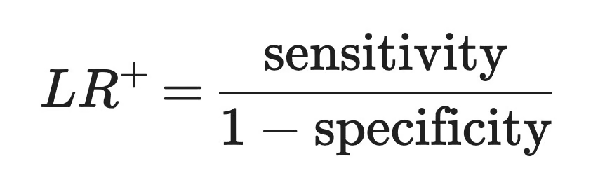
Positive likelihood ratio

For the example test, that's 0.9 / 0.2 = 4.5. A positive result is 4.5 times as likely in someone with the condition. Values above 1 raise the odds of the condition, and the higher the value, the more a positive result tells you.

Negative likelihood ratio

The negative likelihood ratio, or LR-, shows how likely a negative result is among people with the condition compared to people without it:

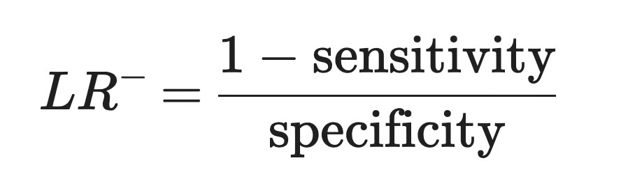
Negative likelihood ratio

For the example test, that's 0.1 / 0.8 = 0.125. Values below 1 lower the odds of the condition, and the closer the value is to 0, the more a negative result tells you.

From pre-test to post-test odds

Diagnostic likelihood ratios are useful because they update what you knew before the test:

Diagnostic likelihood ratio

Let's say 10% of patients like this one have the condition. That's pre-test odds of 0.1 / 0.9, or about 0.111.

After a positive result, the odds become 0.111 * 4.5 = 0.5, which is a probability of about 33%. After a negative result, they become 0.111 * 0.125 = 0.014, or about 1.4%.

This is the one place in the article where a likelihood ratio leads to the probability of a hypothesis, and it's only possible because the pre-test odds supply the prior.

Likelihood Ratio Tests in Python and R

Both languages have everything you need to run an LRT in a couple of lines. I'll use the churn dataset mentioned earlier, so the numbers match the ones in the interpretation and regression sections.

Likelihood ratio test in Python

You'll need numpy, pandas, statsmodels, and scipy. Start by generating the dataset:

import numpy as np
import pandas as pd
import statsmodels.formula.api as smf
from scipy import stats

# Generate a synthetic customer churn dataset
rng = np.random.default_rng(42)
n_customers = 1000

churn = pd.DataFrame({
    "tenure_months": rng.integers(1, 73, n_customers),
    "monthly_charges": rng.uniform(20, 120, n_customers).round(2),
    "support_tickets": rng.poisson(1.5, n_customers),
})

# Churn gets less likely with tenure and more likely with charges and tickets
log_odds = (
    -0.5
    - 0.04 * churn["tenure_months"]
    + 0.01 * churn["monthly_charges"]
    + 0.25 * churn["support_tickets"]
)
churn["churned"] = rng.binomial(1, 1 / (1 + np.exp(-log_odds)))

# Save the data so you can load the same dataset in R
churn.to_csv("churn.csv", index=False)

In this dataset, the churn ratio is 32.1%.

Next, fit the restricted and full logistic regression models. The .llf attribute holds the maximized log-likelihood of each one:

# Fit the restricted and full models
reduced_model = smf.logit("churned ~ tenure_months", data=churn).fit(disp=0)
full_model = smf.logit(
    "churned ~ tenure_months + monthly_charges + support_tickets",
    data=churn,
).fit(disp=0)

# Get the maximized log-likelihoods
print(f"Restricted model log-likelihood: {reduced_model.llf:.2f}")
print(f"Full model log-likelihood: {full_model.llf:.2f}")

Restricted and full model log likelihood

statsmodels doesn't have a general LRT function for logistic regression, so you calculate the statistic from the two log-likelihoods. The .df_model attribute gives the number of predictors in each model, and stats.chi2.sf() returns the p-value:

lr_stat = 2 * (full_model.llf - reduced_model.llf)
df_diff = full_model.df_model - reduced_model.df_model
p_value = stats.chi2.sf(lr_stat, df_diff)

print(f"LR statistic: {lr_stat:.2f}")
print(f"Degrees of freedom: {df_diff:.0f}")
print(f"P-value: {p_value:.1e}")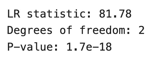

Test statistic, degrees of freedom, and p-value

The p-value is far below 0.05, so you reject the null hypothesis. The data give strong evidence that monthly_charges and support_tickets improve the fit over a model with tenure_months only.

For the comparison against an intercept-only model, you don't need any extra code. statsmodels calculates it for every logistic regression model:

print(f"Intercept-only log-likelihood: {full_model.llnull:.2f}")
print(f"LR statistic: {full_model.llr:.2f}")
print(f"P-value: {full_model.llr_pvalue:.1e}")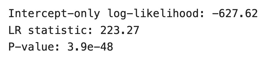

Comparison of a full model to an intercept-only model

Likelihood ratio test in R

R doesn't use the same random number generator as NumPy, so load the churn.csv file from the Python example to work with identical data. Then fit both models with glm() and pass them to anova():

# Load the churn dataset saved from Python
churn <- read.csv("churn.csv")

# Fit the restricted and full models
reduced_model <- glm(churned ~ tenure_months, data = churn, family = binomial)
full_model <- glm(
  churned ~ tenure_months + monthly_charges + support_tickets,
  data = churn,
  family = binomial
)

# Check the maximized log-likelihoods
logLik(reduced_model)
logLik(full_model)

# Run the likelihood ratio test
anova(reduced_model, full_model, test = "Chisq")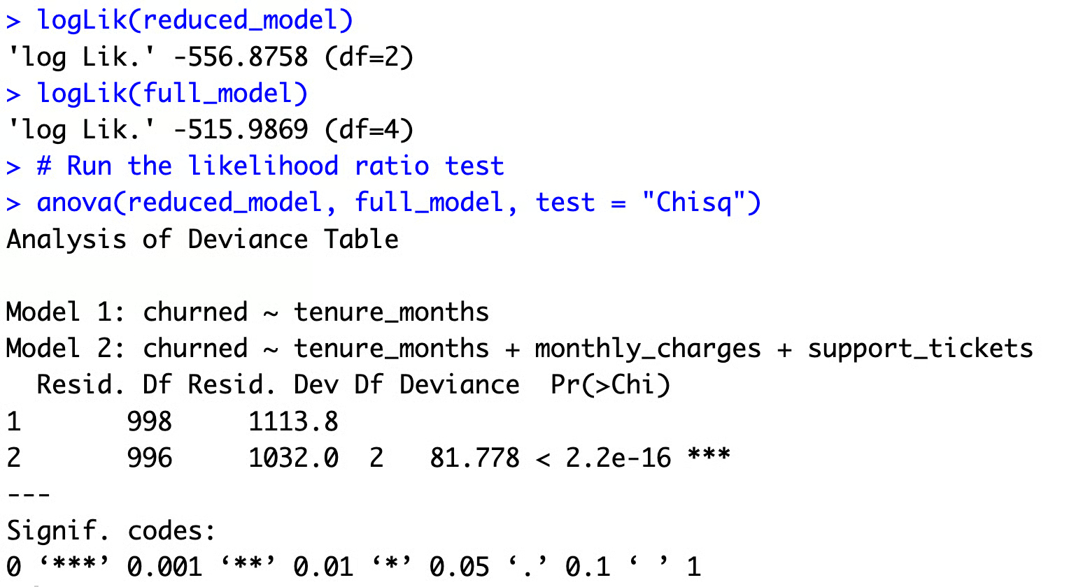

Log likelihoods and ratio test in R

The df values next to each log-likelihood are the number of estimated parameters, intercept included. The full model has two more, which matches the Df column in the anova() table.

The Deviance column shows 81.778, the same LR statistic you got in Python. That's the analysis of deviance from the GLM section in action - the drop in residual deviance from 1113.8 to 1032.0 is the test statistic.

R prints the p-value as < 2.2e-16 because that's the smallest value it shows by default, not because it differs from the Python result. Either way, the conclusion is the same, and the extra predictors improve the fit.

If you prefer a dedicated function, lrtest() from the lmtest package runs the same comparison with lrtest(reduced_model, full_model).

Assumptions and Limitations of Likelihood Ratio Tests

The LRT works well in the settings covered so far, but its chi-square result depends on a couple of conditions.

Models need to be nested

The standard LRT only compares nested models, where the restricted model is a special case of the full one.

If you want to compare a logistic regression with a probit model, or two models with different predictors, neither is a special case of the other. The chi-square distribution doesn't apply there. Use information criteria like AIC and BIC, or the Vuong test for non-nested models, instead.

Both models need maximum likelihood estimates

The test compares maximized likelihoods, so both models have to be fit by maximum likelihood on the same data.

Two common things can go wrong here. Mixed-effects models fit with REML, the default in many packages, can't be compared with an LRT when they differ in fixed effects - so refit them with maximum likelihood first. And penalized models like lasso or ridge regression don't maximize the likelihood itself, so the usual test doesn't apply to them.

The models also need the same observations. If one predictor has missing values, the full model may drop rows, and the two log-likelihoods are no longer comparable.

The chi-square result is asymptotic

Wilks' theorem is a large-sample result. It holds under regularity conditions, which in plain terms mean the likelihood is smooth, the parameters are identifiable, and the true parameter values are inside the allowed range rather than on its edge.

When these conditions are true, the chi-square distribution is a good approximation for large samples. It's still an approximation.

Small samples

With small samples, the LRT statistic may not follow a chi-square distribution, and the p-values can be too small or too large.

You have a couple of options here. A parametric bootstrap simulates new datasets from the restricted model and builds the distribution of the statistic. For simple cases, like contingency tables, exact tests avoid the approximation.

Parameters on the boundary

Some null hypotheses place a parameter on the edge of its allowed range. The most common example is testing whether a random-effect variance in a mixed model equals 0, since a variance can't be negative.

In this case, the statistic doesn't follow the usual chi-square distribution. For a single variance component, it follows a 50:50 mixture of a chi-square with 0 and 1 degrees of freedom, so the standard p-value is about twice as large as it should be. The standard test is conservative here, which means it misses real effects more often.

Testing the number of components in a mixture model has a similar problem. When you compare one component with two, the regularity conditions fail, and the chi-square approximation doesn't hold at all.

Model misspecification

The LRT assumes the full model is correct. If both models get the distribution of the data wrong, like a Poisson model for counts with much more variance than the mean, the statistic won't follow a chi-square distribution even in large samples.

Check the fit of your full model before you trust the test. For overdispersed counts, a negative binomial model or a quasi-likelihood F-test is often a better choice.

So the chi-square approximation is a default, not a guarantee, and it only applies when the setup matches the conditions behind Wilks' theorem.

Conclusion

A likelihood ratio compares how well two hypotheses or models explain the same observed data. That's the whole idea, and everything else in this article builds on it.

The likelihood ratio test makes that idea into a formal procedure. It fits two nested models, compares their maximized log-likelihoods, and uses the chi-square distribution to get a p-value. You'll see it most often in logistic regression and other GLMs, and both statsmodels and R run it with a couple of lines of code.

But remember what the number means. A likelihood ratio shows relative support for one hypothesis over another, not the probability that either one is true. To get that, you need prior odds, like in diagnostic testing.

If you want to go further, the next steps are the building blocks behind the test: likelihood itself, maximum likelihood estimation, and how the Wald test and other hypothesis tests compare to the LRT.