Introduction to Maximum Likelihood Estimation (MLE)

Estimating parameters is a fundamental step in statistical analysis and machine learning. Among the various methods available, Maximum Likelihood Estimation (MLE) is one of the most widely used approaches due to its intuitive nature, mathematical rigor, and broad applicability across different types of data and models.

In this article, you'll learn what MLE is, explore its mathematical foundations through detailed derivations and examples, and discover practical computational methods for implementing MLE effectively.

What is Maximum Likelihood Estimation (MLE)?

Maximum likelihood estimation (MLE) is an important statistical method used to estimate the parameters of a probability distribution by maximizing the likelihood function.

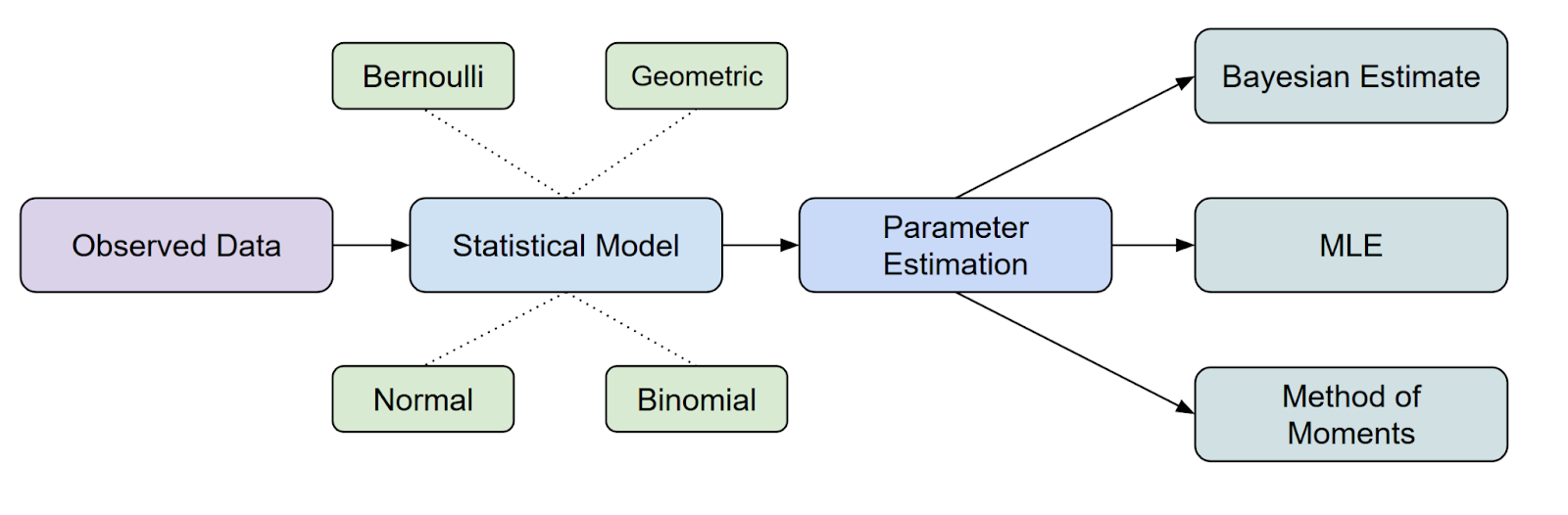
In terms of where MLE fits in statistical inference, it is one of the most common methods we have to estimate parameters.

However, here you might have another question. What is a likelihood function? Let's discuss this further.

What is the Likelihood Function?

We can think of the likelihood function as a way to measure how well a particular set of parameters explains the data you have observed.

In other words, it answers the question: “Given these parameter values, how likely is it that I would see this data?” But there is a common misconception here between Probability and Likelihood:

• Probability is about predicting data from parameters
• Likelihood measures how plausible different parameter values are, given the observed data. It’s a function of parameters for fixed data. In contrast, probability is a function of data for fixed parameters.

Thus, to summarize, the likelihood function takes the parameters of your model as input and gives you a number that represents how plausible those parameters are, given your data.

The higher the value of the likelihood function, the better those parameters explain your data.

To put it even more simply, the likelihood function helps us “score” different parameter choices, so we can pick the ones that make our observed data most probable.

Now that we have understood the difference between Probability and Likelihood, as well as what MLE is used for, let's proceed to the underlying mathematics.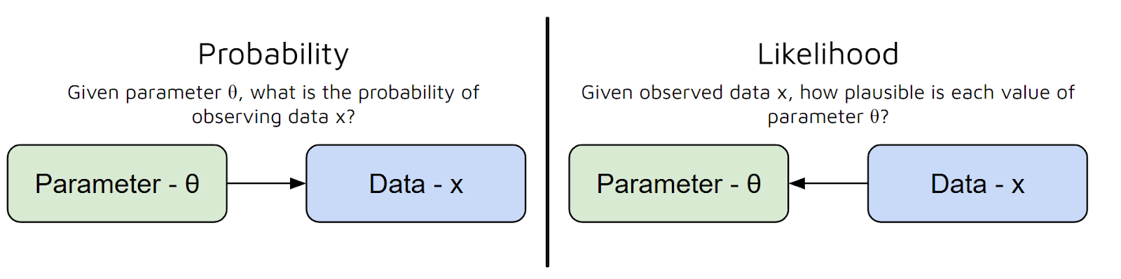 

How to Derive the MLE Formula

Before we jump into specific examples, let’s see how the maximum likelihood estimator (MLE) is derived in general. We will go through each step and also explain the reasoning behind it.

Step 1: Define probability model

Let’s suppose we have a dataset: x₁, x₂, ..., xₙ. We believe these data points are generated from a probability distribution that depends on some unknown parameter θ (theta). Our main goal is to estimate θ. 

For example, if our dataset were about coin flips, θ could be the probability of heads. If the dataset were continuous, like the heights of students in the class, θ could be the mean of a normal distribution.

Step 2: Writing the likelihood function

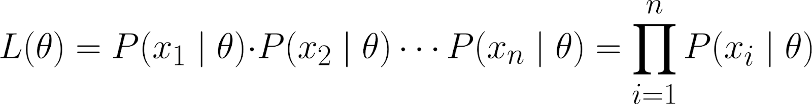
The likelihood function measures how likely it is to observe your data for different values of θ. It is defined as:

Intuitively, we are asking, given that the parameter θ takes a specific value, what is the probability of observing this particular dataset? 

This dataset is represented as the joint probability of observing the individual data points (x₁, x₂, ..., xₙ), assuming they were generated under the model parameterized by θ. 

Using the chain rule of probability, we can expand the above equation into this:

However, this is quite a complicated equation! So we make the assumption that the data points are independent - more specifically, conditionally independent. 

By doing so, we can get the joint probability to be the product of individual probabilities:

Since our observed data points are conditionally independent on θ, we know the following equation is true:

This is because we have assumed that once we know the value of θ, the data points x₁ and x₂ are conditionally independent.

Step 3: Find the value of θ that maximizes likelihood

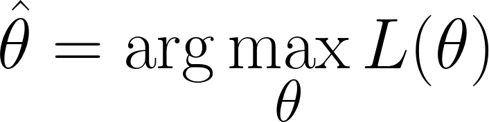
We are in the position where we have to find the values of θ which maximizes the likelihood function(i.e, it makes the observed data most likely):

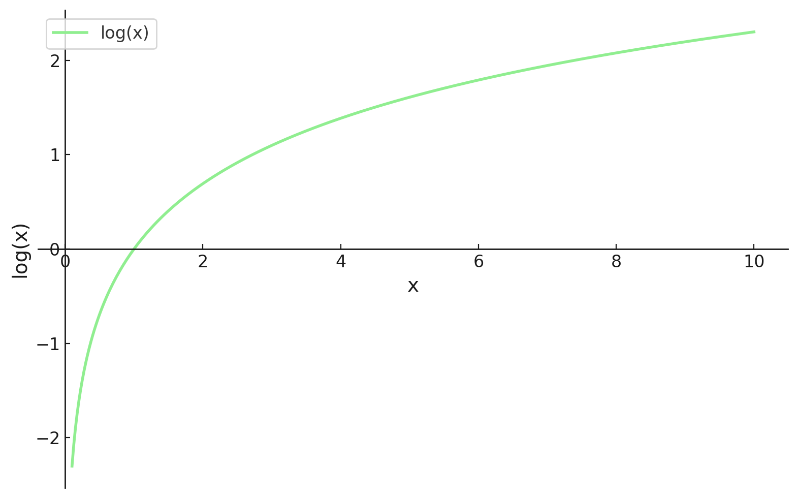
However, recall that our likelihood function contains a product. Working with products can get messy, especially with lots of data points. To simplify, we take the logarithm of the likelihood function since this converts the product into a summation.

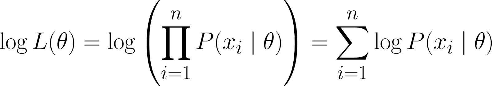
This gives us the log-likelihood, which has some beneficial properties:

• The log turns products into sums, which are much easier to work with, especially when differentiating.
• The log function is monotonic, so maximizing the log-likelihood gives the same θ as maximizing the likelihood.

Step 4: Finding the optimal value

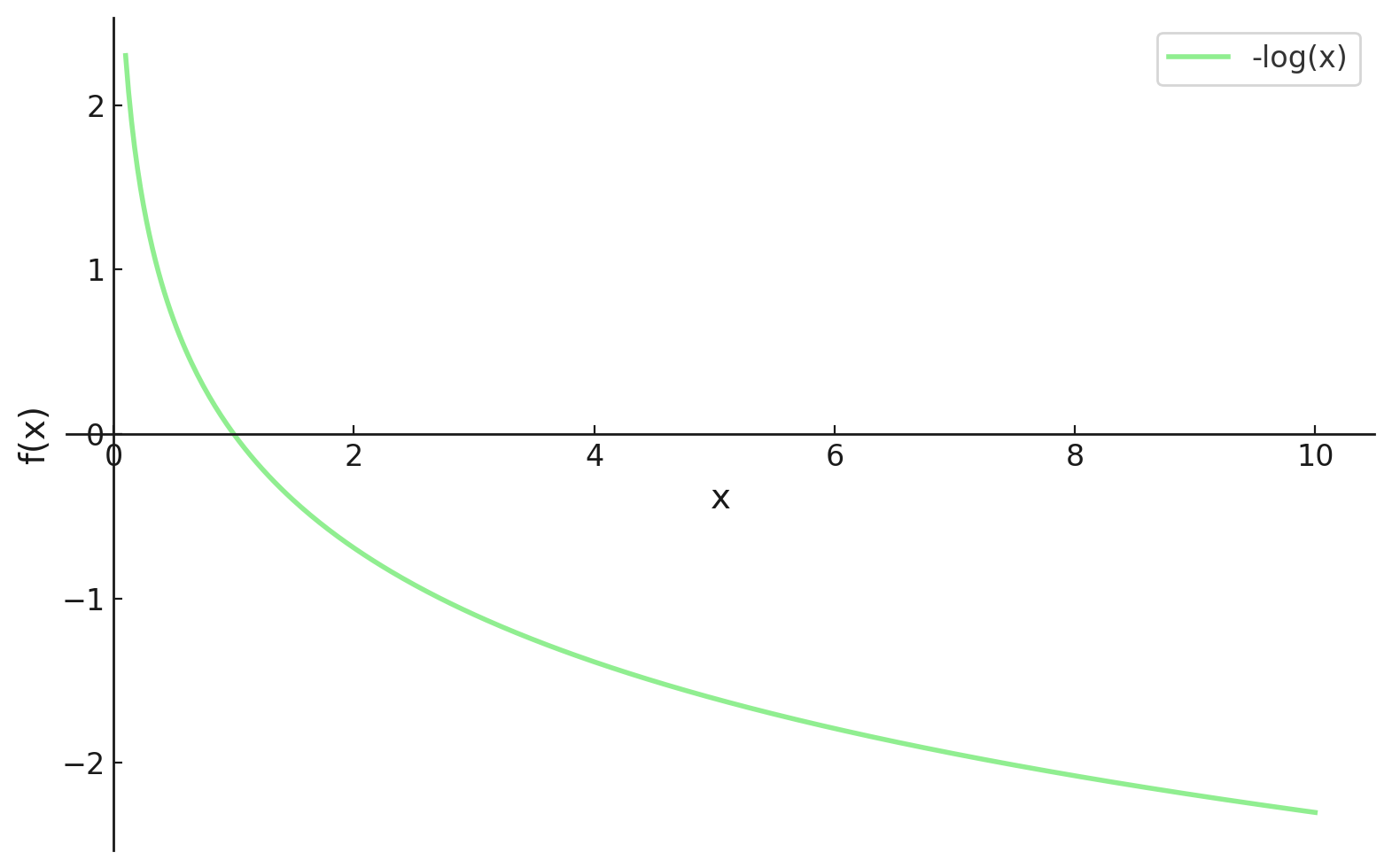
We are now at a place where we can differentiate, however in machine learning, we tend to want our loss functions to be minimized. Luckily, this is quite an easy fix. 

By including a minus symbol (i.e., multiplying by -1) at the start of our function, we now need to minimize our loss function, which is now called the Negative Log-Likelihood Loss Function.

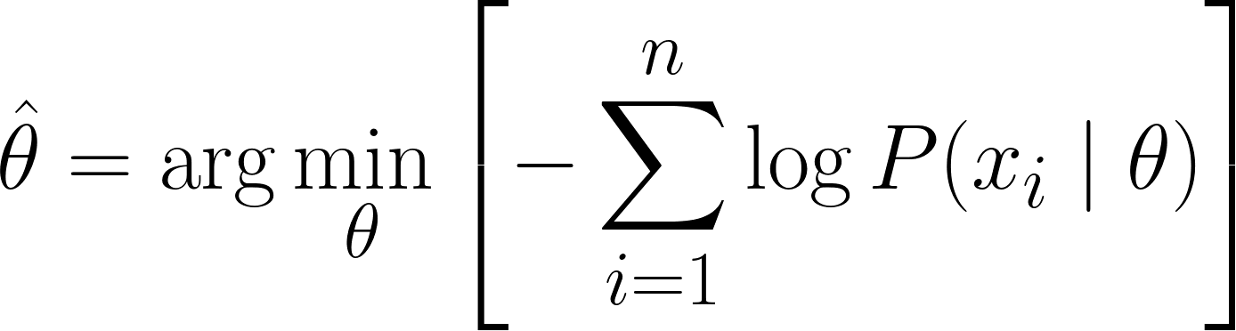
Now, we can use calculus to obtain the value of θ. By taking the derivative of the log-likelihood with respect to θ, setting it to zero, and solving for θ. This is because the minimum of a function occurs where its derivative is zero (and the second derivative is positive).

Therefore, the final equation for MLE is:

Worked MLE Examples

Since we have successfully derived the MLE Equation, let's look at some worked examples to solidify our understanding.

Dice rolls example

Let’s start with a simple, discrete example: estimating the probability of rolling a six with a possibly biased die.

Suppose we roll a die 12 times and record the results. We want to model this data using a categorical distribution, but let’s focus on estimating the probability θ (theta) of rolling a six. In this example:

• Parameter (θ): The value you want to estimate - Probability of rolling a six
• Data (x): The results we observed - 4 sixes out of 12 rolls

Now we calculate the Likelihood function, which, because we got 4 sixes out of 12 rolls, we would obtain:

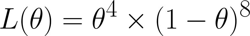
We obtained this since out of the 12 times, we obtain sixes 4 times - hence we have θ⁴ and we obtained non-sixes 8 times - hence we have the (1 - θ)⁸ term. 

Recall, we have multiplied these since we have assumed that these are conditionally independent. 

Now we take the negative log-likelihood as we previously discussed, giving us this equation:

Finally, we differentiate the equation with respect with θ and set it to 0 (since we want to find the minimum point):

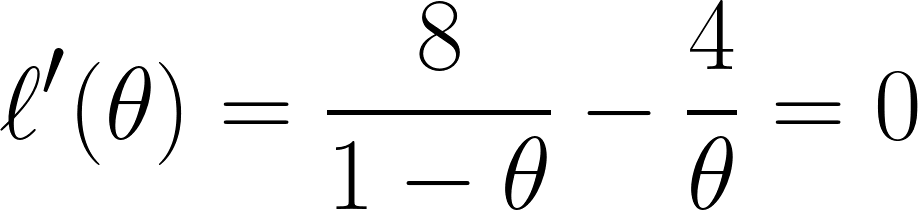
And through this equation, we can conclude that θ is equal to ⅓ . 

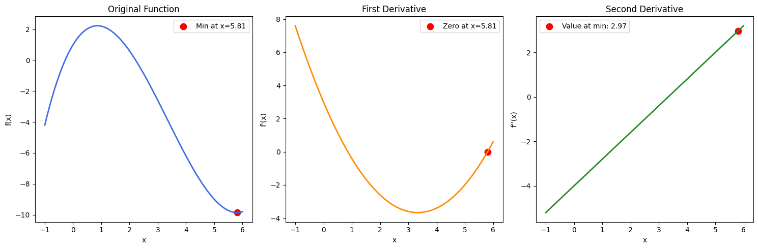
Note: If we had obtained multiple solutions of θ, then we would have to also find the second derivative and see which θ values would give us a positive result (to confirm we have found a minimum point). This can be confirmed through an example function in the image below:

Heights example

Let’s now look at a continuous example - estimating the mean of a normal (Gaussian) distribution.

Lets suppose we have a dataset of the heights of 5 people: 160, 165, 170, 175, 180 (in cm). We will also assume these are drawn from a normal distribution with unknown mean μ (mu) and known variance σ² (let’s say σ² = 25 for simplicity).

• Parameter (μ): The value you want to estimate (the average height)
• Data (x₁, x₂, ..., x₅): The observed heights

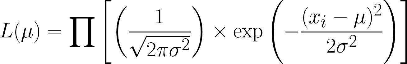
The likelihood function for the normal distribution (with known variance) is. 

This is very complicated but taking the negative log makes things easier. Hopefully, you can now see the power of using the log function in our equation. The equation we obtain is this:

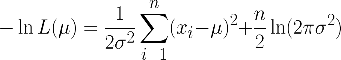
We obtain two terms here, but note how the second term can be disregarded when we proceed with differentiation, since we are differentiating with respect to μ, and the second term does not contain μ. 

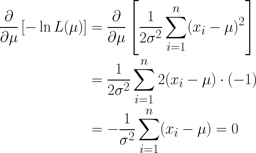
We are almost there, but take a look at μ in the brackets. 

Since it is a constant, we can simply multiply it by n, since adding μ n-times, will simply be n*μ. 

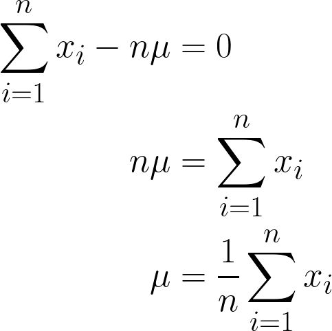
The final answer we have obtained should make intuitive sense, since it is mathematically stated to sum all values of x and divide by n (which is the number of observations we have), and this is also the mean’s definition!

Thus, by putting in our data values to this equation, we can obtain the mean to be 170cm. 

To make this more visual, here is an animation showing how the likelihood changes as we change μ:

In both examples, using MLE gave us the parameter value that made our observed data most probable under the chosen model. Obviously, MLE can work with giving us multiple parameter values as well, although the calculation would be slightly longer!

Coding MLE

Now that we have understood the underlying structure of MLE, let’s see how to code this in Python. We will be coding the previous example (heights) solution. 

# Importing libraries 
import numpy as np # used for handling arrays and mathematical operations.
from scipy.optimize import minimize # function that minimizes another function

# This is our sample data 
data = np.array([160, 165, 170, 175, 180])

# This was the variance we had assumed before
sigma_squared = 25

# Negative Log-Likelihood function
def negative_log_likelihood(mu):
    n = len(data) # Number of data points
    return 0.5 * n * np.log(2 * np.pi * sigma_squared) + \
           np.sum((data - mu)**2) / (2 * sigma_squared) # The NLL is for the Univariate Gaussian Distribution

# Optimizing the NLL
result = minimize(negative_log_likelihood, x0=170)  # initial guess

# Our final estimated mean
estimated_mu = result.x[0]
print(f"MLE estimate of mu: {estimated_mu}")

Computational Strategies and Algorithms

Notice when we were coding the previous example, we had created a function negative_log_likelihood() which contained the main logic for calculating the MLE of a Univariate Gaussian Distribution. 

On the one hand, it could be argued that we ultimately hard-coded this equation, and we used the scipy.optimize to minimize that function. Of course, this is still a completely viable solution, since the Gaussian Distribution has a closed form solution. 

Let’s explore other methods to compute solutions for MLE.

Closed-form solutions and when they apply

As we discussed above, in some fortunate cases, we can solve the MLE equations analytically, which means we can derive an exact formula for the parameter estimates. These are known as closed-form solutions, and they are often simple, intuitive, and fast to code and compute.

An important question to ask now is, when do closed-form solutions exist?

1. When the log-likelihood function is differentiable, concave, and algebraically tractable.
2. When the model is simple enough; typically involving one or two parameters and no hidden variables.

Numerical optimization techniques

For more complex models, analytical solutions don't exist or are too complicated to derive. In these cases, we use numerical optimization methods - iterative algorithms that search for the parameters that maximize the log-likelihood. Let’s briefly explain them:

1. Newton-Raphson method: This method uses both:

• The first derivative (gradient) to determine the slope, and
• The second derivative (Hessian) to gauge curvature and adjust the step size accordingly.
• The update rule is such:
• Its main benefit is that it has fast convergence near the optimum.
• However, it requires computing second derivatives, which can be unstable or expensive in high dimensions.

2. Quasi-Newton methods (e.g., BFGS):

• Approximate the Hessian matrix using only first-order derivatives
• Used in popular libraries like scipy.optimize.minimize in Python (with BFGS as the default).
• More numerically stable and broadly applicable than Newton-Raphson.

3. Expectation-Maximization (EM) algorithm:

• Specialized optimization technique used when the data involves latent (hidden) variables—values we don’t observe directly but that influence the data.
• There are two steps in this algorithm:
• E-step (Expectation): Compute the expected value of the log-likelihood using the current estimates of the parameters and observed data.
• M-step (Maximization): Maximize this expected log-likelihood to update the parameter estimates.

Properties of MLE

From our examples and calculations, it is clear that MLE is useful. Formally speaking, MLE has the following properties: 

1. Consistency: As the sample size increases, the MLE converges to the true value of the parameter.
2. Asymptotic Normality: For large samples, the distribution of the MLE becomes approximately normal (bell-shaped) around the true parameter value. This is the basis for constructing confidence intervals.
3. Efficiency: Among all unbiased estimators, the MLE achieves the lowest possible variance (it reaches the Cramér-Rao lower bound, at least asymptotically).
4. Invariance: If θ̂ is the MLE for θ, then for any function g, g(θ̂) is the MLE for g(θ). In other words, MLEs are preserved under transformations.

However, there are scenarios where using MLE might not be the best option:

1. Small samples: MLE can be biased when the sample size is small. For example, the MLE for variance (σ̂²) tends to underestimate the true variance (σ²).
2. Robustness: MLE is sensitive to outliers and model misspecification. Alternatives like M-estimators can provide more robust estimates.
3. Bayesian alternative: Maximum a posteriori (MAP) estimation combines prior information with the likelihood, offering a Bayesian perspective and sometimes more stable estimates, especially with limited data.

Applications Across Statistical Modeling

In this section, let’s explore where MLE is actually used in Machine Learning and AI.

Regression and classification

One of the most important places MLE appears is in logistic regression. Here, we are estimating the probability that an outcome belongs to a certain class (such as customer churn) and we do this by fitting parameters to maximize the likelihood of the observed outcomes.

Even in linear regression, if we assume normally distributed errors, then the least squares solution actually turns out to be the MLE too. 

Hypothesis testing and model selection

MLE can also be used to compare models. 

For example, the likelihood ratio test (LRT) helps us check if adding extra variables to a model significantly improves its performance. It works by comparing the likelihoods of two models: one simpler (null), one more complex (alternative).

We also have the Akaike Information Criterion (AIC), which penalizes complexity to avoid overfitting. These tools are widely used in fields like finance, medicine, and marketing.

If you're interested in further exploring ways to measure differences between probability distributions beyond likelihood alone, check out my tutorial: KL-Divergence Explained.

Limitations and Alternatives to MLE

Although it is powerful, it does have its drawbacks. Let's quickly go over where it struggles, and what we can use instead.

Key limitations of MLE

• Sensitive to model misspecification: If our model is wrong (e.g., using a normal distribution for skewed data), MLE will give us misleading results.
• Outlier sensitivity: A few bad data points can completely throw off your estimates.
• Computational cost: For large models, especially with many parameters or constraints, optimizing the likelihood can be slow or unstable.
• Multiple solutions: Sometimes the likelihood surface has several peaks (local maxima), which makes finding the best solution tricky.

Alternatives to maximum likelihood estimation

When MLE doesn’t work well, here are some options:

• MAP (Maximum a Posteriori): Like MLE, but adds a prior belief. This can help stabilize estimates when data is limited.
• Method of Moments: Matches sample moments (like the mean or variance) with theoretical ones. It’s less precise than MLE but very easy to compute.
• Least Squares: In cases like linear regression with Gaussian errors, least squares and MLE are the same. But least squares can still be useful when MLE is too complex.

Different methods work better in different situations. MLE might not always be the answer, but it’s often a great starting point.

Conclusion

Maximum Likelihood Estimation is one of the most natural and widely used methods for parameter estimation. It is the idea of making the observed data as probable as possible, and thus can be used in many different scenarios, such as coin flips, Gaussian heights, etc. 

MLE can adapt across models and scale with data, offering both mathematical elegance and practical power. Although it does have its own drawbacks, especially in small or messy datasets, it remains a foundational tool when learning Machine Learning and AI. 

If you’re on your machine learning journey, be sure to check out our Machine Learning Scientist in Python career track, which explores supervised, unsupervised, and deep learning. 

Ready to deepen your understanding of Maximum Likelihood Estimation with practical exercises? These resources can help you apply your knowledge and gain hands-on experience:

• Maximizing Likelihood, Part 1 (Python): Compute and visualize log-likelihoods to clearly see how parameter estimates are determined in practice.
• OLS Regression: The Key Ideas Explained: Explore the connection between Ordinary Least Squares regression and MLE when assuming Gaussian errors, reinforcing core statistical concepts.
• Understanding Logistic Regression in Python: Delve into how logistic regression leverages MLE for effective classification and parameter estimation.