Introduction to Regression with statsmodels in Python
BeginnerSkill Level
4 hr
41.5K learners
Practice Lasso and Ridge Regression in Python with this hands-on exercise.
Linear regression is a type of linear model that is considered the most basic and commonly used predictive algorithm. This can not be dissociated from its simple, yet effective architecture. A linear model assumes a linear relationship between input variable(s) 𝑥 and an output variable y. The equation for a linear model looks like this:
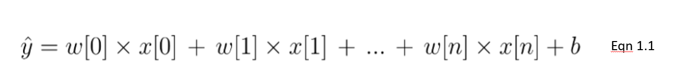
In this equation 1.1, we show a linear model with n number of features. w is considered the coefficient (or weights) assigned to each feature - an indicator of their significance to the outcome y. For example, we assume that temperature is a larger driver of ice cream sales than whether it's a public holiday. The weight assigned to temperature in our linear model will be larger than the public holiday variable.
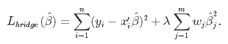
The goal for a linear model then becomes to optimize the weight (b) via the cost function in equation 1.2. The cost function calculates the error between predictions and actual values, represented as a single real-valued number. The cost function is the average error across n samples in the dataset, represented below as:
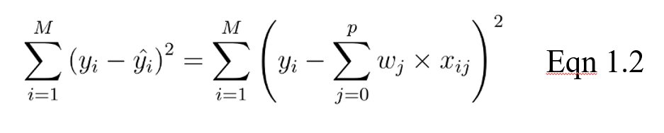
In the equation above, yi is the actual value and that is the predicted value from our linear equation, where M is the number of rows and P is the number of features.
When it comes to training models, there are two major problems one can encounter: overfitting and underfitting.
Particularly, regularization is implemented to avoid overfitting of the data, especially when there is a large variance between train and test set performances. With regularization, the number of features used in training is kept constant, yet the magnitude of the coefficients (w) as seen in equation 1.1, is reduced.
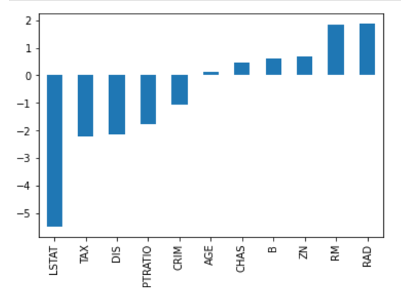
Consider the image of coefficients below to predict house prices. While there are quite a number of predictors, RM and RAD have the largest coefficients. The implication of this will be that housing prices will be driven more significantly by these two features leading to overfitting, where generalizable patterns have not been learned.
There are different ways of reducing model complexity and preventing overfitting in linear models. This includes ridge and lasso regression models.
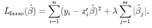
This is a regularization technique used in feature selection using a Shrinkage method also referred to as the penalized regression method. Lasso is short for Least Absolute Shrinkage and Selection Operator, which is used both for regularization and model selection. If a model uses the L1 regularization technique, then it is called lasso regression.
In this shrinkage technique, the coefficients determined in the linear model from equation 1.1. above are shrunk towards the central point as the mean by introducing a penalization factor called the alpha α (or sometimes lamda) values.
Alpha (α) is the penalty term that denotes the amount of shrinkage (or constraint) that will be implemented in the equation. With alpha set to zero, you will find that this is the equivalent of the linear regression model from equation 1.2, and a larger value penalizes the optimization function. Therefore, lasso regression shrinks the coefficients and helps to reduce the model complexity and multi-collinearity.
Alpha (α) can be any real-valued number between zero and infinity; the larger the value, the more aggressive the penalization is.
Due to the fact that coefficients will be shrunk towards a mean of zero, less important features in a dataset are eliminated when penalized. The shrinkage of these coefficients based on the alpha value provided leads to some form of automatic feature selection, as input variables are removed in an effective approach.
Similar to the lasso regression, ridge regression puts a similar constraint on the coefficients by introducing a penalty factor. However, while lasso regression takes the magnitude of the coefficients, ridge regression takes the square.
Ridge regression is also referred to as L2 Regularization.
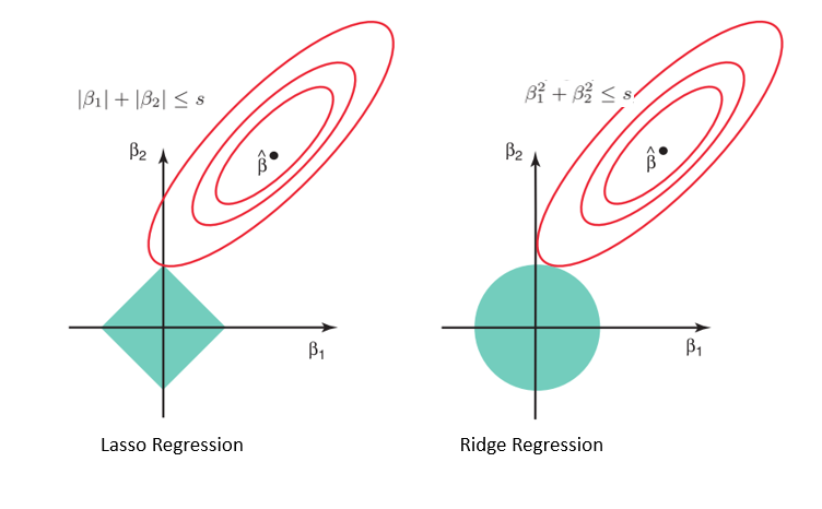
Considering the geometry of both the lasso (left) and ridge (right) models, the elliptical contours (red circles) are the cost functions for each. Relaxing the constraints introduced by the penalty factor leads to an increase in the constrained region (diamond, circle). Doing this continually, we will hit the center of the ellipse, where the results of both lasso and ridge models are similar to a linear regression model.
However, both methods determine coefficients by finding the first point where the elliptical contours hit the region of constraints. Since lasso regression takes a diamond shape in the plot for the constrained region, each time the elliptical regions intersect with these corners, at least one of the coefficients becomes zero. This is impossible in the ridge regression model as it forms a circular shape and therefore values can be shrunk close to zero, but never equal to zero.
For this implementation, we will use the Boston housing dataset found in Sklearn. What we intend to see is:
#libraries
import pandas as pd
import numpy as np
import seaborn as sns
import matplotlib.pyplot as plt
from sklearn.model_selection import train_test_split
from sklearn.linear_model import LinearRegression
from sklearn.linear_model import Ridge, RidgeCV, Lasso
from sklearn.preprocessing import StandardScaler
from sklearn.datasets import load_boston

#data
boston = load_boston()
boston_df=pd.DataFrame(boston.data,columns=boston.feature_names)
#target variable
boston_df['Price']=boston.target
#preview
boston_df.head()

#Exploration
plt.figure(figsize = (10, 10))
sns.heatmap(boston_df.corr(), annot = True)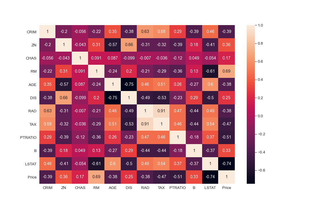
#There are cases of multicolinearity, we will drop a few columns
boston_df.drop(columns = ["INDUS", "NOX"], inplace = True)

#pairplot
sns.pairplot(boston_df)

#we will log the LSTAT Column
boston_df.LSTAT = np.log(boston_df.LSTAT)
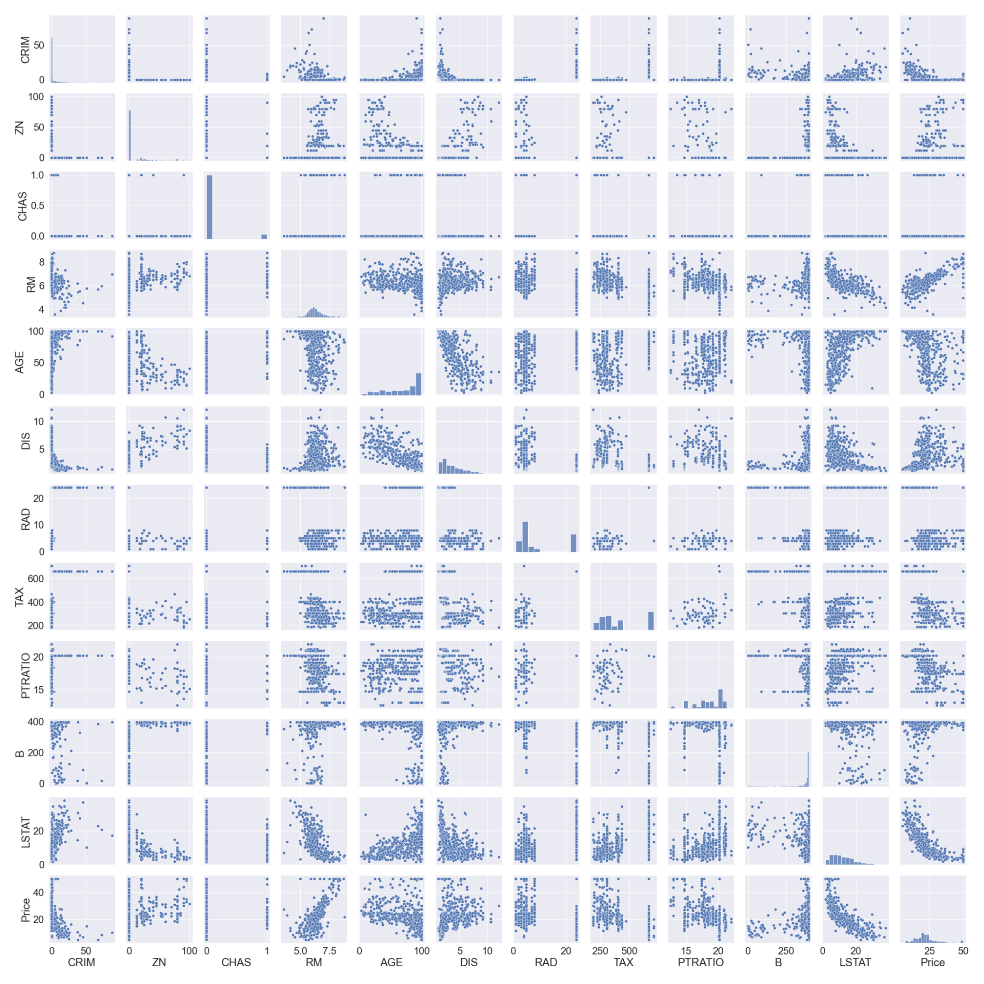
Note that we logged the LSTAT column as it doesn’t have a linear relationship with the price column. Linear models assume a linear relationship between x and y variables.
#preview
features = boston_df.columns[0:11]
target = boston_df.columns[-1]
#X and y values
X = boston_df[features].values
y = boston_df[target].values
#splot
X_train, X_test, y_train, y_test = train_test_split(X, y, test_size=0.3, random_state=17)
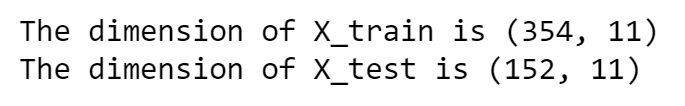
print("The dimension of X_train is {}".format(X_train.shape))
print("The dimension of X_test is {}".format(X_test.shape))
#Scale features
scaler = StandardScaler()
X_train = scaler.fit_transform(X_train)
X_test = scaler.transform(X_test)
Output:
We will build a linear and a ridge regression model and then compare the coefficients in a plot. The score of the train and test sets will also help us evaluate how well the model performs.
#Model
lr = LinearRegression()

#Fit model
lr.fit(X_train, y_train)

#predict
#prediction = lr.predict(X_test)

#actual
actual = y_test

train_score_lr = lr.score(X_train, y_train)
test_score_lr = lr.score(X_test, y_test)

print("The train score for lr model is {}".format(train_score_lr))
print("The test score for lr model is {}".format(test_score_lr))


#Ridge Regression Model
ridgeReg = Ridge(alpha=10)

ridgeReg.fit(X_train,y_train)

#train and test scorefor ridge regression
train_score_ridge = ridgeReg.score(X_train, y_train)
test_score_ridge = ridgeReg.score(X_test, y_test)

print("\nRidge Model............................................\n")
print("The train score for ridge model is {}".format(train_score_ridge))
print("The test score for ridge model is {}".format(test_score_ridge))
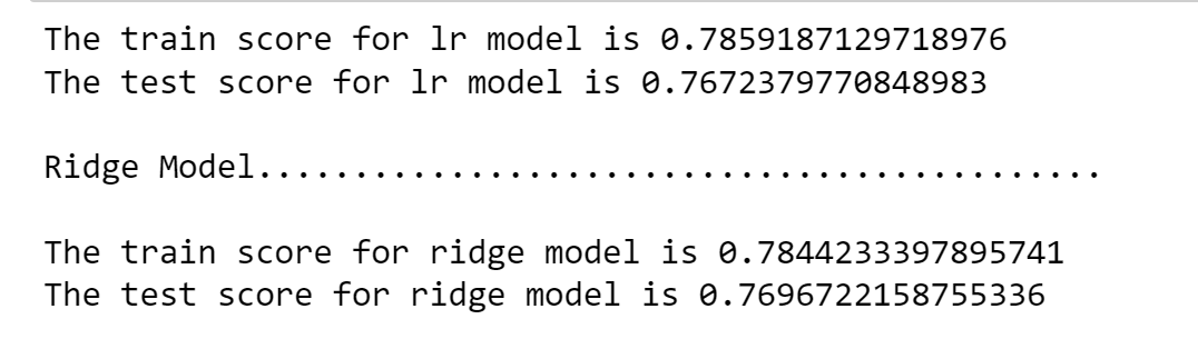
Using an alpha value of 10, the evaluation of the model, the train, and test data indicate better performance on the ridge model than on the linear regression model.
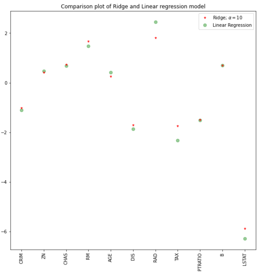
We can also plot the coefficients for both the linear and ridge models.
plt.figure(figsize = (10, 10))
plt.plot(features,ridgeReg.coef_,alpha=0.7,linestyle='none',marker='*',markersize=5,color='red',label=r'Ridge; $\alpha = 10$',zorder=7)
#plt.plot(rr100.coef_,alpha=0.5,linestyle='none',marker='d',markersize=6,color='blue',label=r'Ridge; $\alpha = 100$')
plt.plot(features,lr.coef_,alpha=0.4,linestyle='none',marker='o',markersize=7,color='green',label='Linear Regression')
plt.xticks(rotation = 90)
plt.legend()
plt.show()
#Lasso regression model
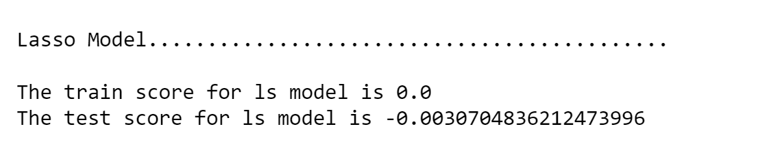
print("\nLasso Model............................................\n")
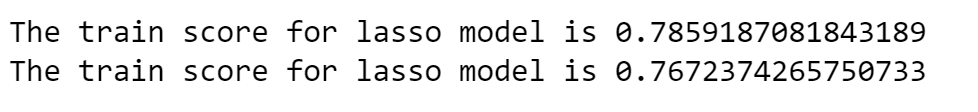
lasso = Lasso(alpha = 10)
lasso.fit(X_train,y_train)
train_score_ls =lasso.score(X_train,y_train)
test_score_ls =lasso.score(X_test,y_test)
print("The train score for ls model is {}".format(train_score_ls))
print("The test score for ls model is {}".format(test_score_ls))
We can visualize the coefficients too.
pd.Series(lasso.coef_, features).sort_values(ascending = True).plot(kind = "bar")
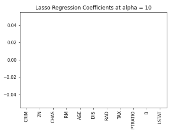
Earlier on, we established that the lasso model can inert to zero due to the diamond shape of the constraint region. In this case, using an alpha value of 10 over penalizes the model and shrinks all the values to zero. We can see this effectively by visualizing the coefficients of the model as shown in the figure above.
We may need to try out different alpha values to find the optimal constraint value. For this case, we can use the cross-validation model in the sklearn package. This will try out different combinations of alpha values and then choose the best model.
#Using the linear CV model
from sklearn.linear_model import LassoCV

#Lasso Cross validation
lasso_cv = LassoCV(alphas = [0.0001, 0.001,0.01, 0.1, 1, 10], random_state=0).fit(X_train, y_train)


#score
print(lasso_cv.score(X_train, y_train))
print(lasso_cv.score(X_test, y_test))
Output:
The model will be trained on different alpha values that I have specified in the LassoCV function. We can observe a better performance of the model, removing the tedious effort of manually changing alpha values.
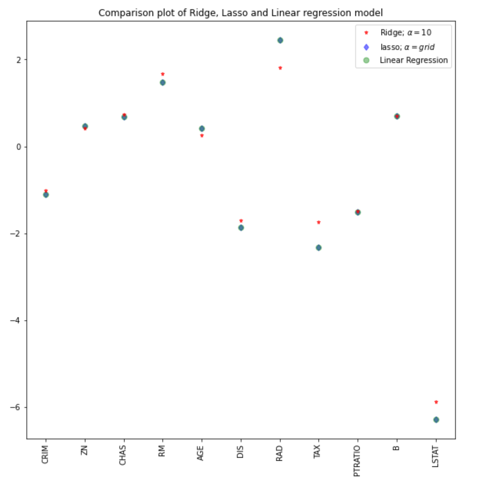
We can compare the coefficients from the lasso model with the rest of the models (linear and ridge).
#plot size
plt.figure(figsize = (10, 10))
#add plot for ridge regression
plt.plot(features,ridgeReg.coef_,alpha=0.7,linestyle='none',marker='*',markersize=5,color='red',label=r'Ridge; $\alpha = 10$',zorder=7)

#add plot for lasso regression
plt.plot(lasso_cv.coef_,alpha=0.5,linestyle='none',marker='d',markersize=6,color='blue',label=r'lasso; $\alpha = grid$')

#add plot for linear model
plt.plot(features,lr.coef_,alpha=0.4,linestyle='none',marker='o',markersize=7,color='green',label='Linear Regression')

#rotate axis
plt.xticks(rotation = 90)
plt.legend()
plt.title("Comparison plot of Ridge, Lasso and Linear regression model")
plt.show()
Note: A similar approach could be employed for the ridge regression model, which could lead to better results. In the sklearn package, the function RidgeCV performs similarly.
#Using the linear CV model
from sklearn.linear_model import RidgeCV

#Lasso Cross validation
ridge_cv = RidgeCV(alphas = [0.0001, 0.001,0.01, 0.1, 1, 10]).fit(X_train, y_train)

#score
print("The train score for ridge model is {}".format(ridge_cv.score(X_train, y_train)))
print("The train score for ridge model is {}".format(ridge_cv.score(X_test, y_test)))
Learn about other kinds of regression with our logistic regression in python and linear regression in python tutorials.
We have seen an implementation of ridge and lasso regression models and the theoretical and mathematical concepts behind these techniques. Some of the key takeaways from this tutorial include:
You can find a more robust and complete notebook for the python implementation here, or do a deep dive into regressions with our Introduction to Regression in Python course.
Tutorial
Michał Oleszak
Tutorial
Sayak Paul
Tutorial
Avinash Navlani
Tutorial
Josef Waples
Tutorial
Zoumana Keita
code-along
George Boorman