Understanding Correlation: Measuring Relationships in Data

If you’ve already explored our tutorial on covariance, you know it’s all about how two variables change together. Correlation takes that concept a step further by standardizing the measure so you can compare relationships across different datasets.

In this guide, you’ll learn what correlation is (specifically, we will focus on the most common one, called Pearson correlation), how it differs from covariance, and how to calculate and interpret it using Python and R. And the end, we’ll also cover different kinds of correlation used for different scenarios.

To continue strengthening your stats skills, don’t miss our Statistics Fundamentals in Python skill track or Introduction to Statistics in R course.

What Is Correlation?

Correlation measures the strength and direction of a linear relationship between two quantitative variables. It helps you understand how changes in one variable are associated with changes in another. 

A positive correlation means that as one variable increases, the other tends to increase as well. A negative correlation means that as one variable increases, the other tends to decrease.

Let me list the main ideas:

• Correlation quantifies the degree to which two variables move together.
• The correlation coefficient ranges from -1 to 1.
• A value of 1 indicates a perfect positive linear relationship.
• A value of -1 indicates a perfect negative linear relationship.
• A value of 0 indicates no linear relationship.

Pearson Correlation Coefficient Formula

As I mentioned, the Pearson correlation coefficient measures the linear relationship between two continuous variables. What I haven’t yet said: It assumes normally distributed data (actually, more exactly, it assumes the variables are jointly normally distributed which is known as bivariate normality - some nuance there), and is sensitive to outliers. The Pearson correlation coefficient is denoted as r.

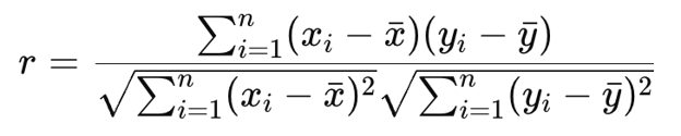
where xi​ and yi​ are data points, and x and y​ are their respective means.

Pearson Correlation Coefficient in Python and R

Let’s see how to calculate in Python and R. 

Correlation in Python

You can calculate the Pearson correlation coefficient in Python using the pearsonr() function from the scipy.stats module:

import numpy as np
from scipy.stats import pearsonr

# Temperature data in Celsius and corresponding Fahrenheit
temperature_celsius = np.array([0, 10, 20, 30, 40])
temperature_fahrenheit = np.array([32, 50, 68, 86, 104])  # Converted from Celsius

# Calculate Pearson correlation coefficient
correlation_coefficient, p_value = pearsonr(temperature_celsius, temperature_fahrenheit)
print("Pearson correlation coefficient:", correlation_coefficient)

Pearson correlation coefficient: 1.0
p-value: 0.0

The output shows a perfect positive linear relationship between x_values and y_values (since we just defined y as 2x). 

Correlation in R

For R, you can use the cor() function:

temperature_celsius <- c(0, 10, 20, 30, 40)
temperature_fahrenheit <- c(32, 50, 68, 86, 104)  # Converted from Celsius

# Calculate Pearson correlation coefficient
correlation_coefficient <- cor(temperature_celsius, temperature_fahrenheit, method = "pearson")
print(correlation_coefficient)

[1] 1

This output also indicates a perfect positive linear relationship, same as before.

Correlation Matrix

A correlation matrix displays the correlation coefficients between multiple pairs of variables in a dataset. It is useful for exploring relationships in multivariate data.

Correlation matrix in Python

It's common to represent variable in a matrix format, like a pandas DataFrame, and compute the correlation matrix directly:

import pandas as pd

# Create a DataFrame with two perfectly correlated variables and one that isn't
data = pd.DataFrame({
    'temperature_celsius': [0, 10, 20, 30, 40],
    'temperature_fahrenheit': [32, 50, 68, 86, 104],  # Perfect linear transformation
    'ice_cream_sales': [100, 150, 200, 220, 230]      # Roughly increasing, not perfectly
})

# Calculate the Pearson correlation matrix
correlation_matrix = data.corr(method='pearson')
print(correlation_matrix)

                      temperature_celsius  temperature_fahrenheit  ice_cream_sales
temperature_celsius              1.000000                1.000000         0.993858
temperature_fahrenheit           1.000000                1.000000         0.993858
ice_cream_sales                  0.993858                0.993858         1.000000

This output shows:

• A perfect positive correlation between temperature_celsius and temperature_fahrenheit (as expected, like before).

• A strong but not perfect correlation between ice_cream_sales and both temperature_celsius and temperature_fahrenheit.

Correlation matrix in R

In R, you can achieve the same with the cor() function we usd before, applied to a data frame or matrix:

# Create a data frame with two perfectly correlated variables and one unrelated
data <- data.frame(
  temperature_celsius = c(0, 10, 20, 30, 40),
  temperature_fahrenheit = c(32, 50, 68, 86, 104),  # Perfect conversion from Celsius
  ice_cream_sales = c(100, 150, 200, 220, 230)      # Generally increases, but not perfectly
)

# Calculate the correlation matrix
correlation_matrix <- cor(data, method = "pearson")
print(correlation_matrix)

                      temperature_celsius temperature_fahrenheit ice_cream_sales
temperature_celsius                 1.00                   1.00            0.99
temperature_fahrenheit              1.00                   1.00            0.99
ice_cream_sales                     0.99                   0.99            1.00

This R output mirrors the Python example, with:

• Perfect positive correlation between temperature_celsius and temperature_fahrenheit.

• Strong negative correlation between ice_cream_sales and temperature_celsius or temperature_fahrenheit.

This kind of matrix view is especially useful for identifying potential multicollinearity in regression or choosing variables for dimensionality reduction techniques like PCA.

Correlation vs. Other Metrics

We see that correlation captures linear associations. Now, let's take some care to clearly distinguish it from similar-sounding ideas.

Correlation vs. covariance

Both correlation and covariance measure how two variables change together, but they are different in two things: scale and interpretability.

• Covariance indicates the direction of a linear relationship but not its strength in a standardized way. Its value depends on the units of the variables, making it hard to compare across datasets.

• Correlation standardizes the covariance by dividing by the standard deviations of the variables, producing a unitless value between -1 and 1.

Correlation vs. R-squared

R-squared (R²), or the coefficient of determination, might also be confused with correlation. I've seen this especially when analysts try to interpret model performance.

• Correlation (Pearson’s r) measures the strength and direction of a linear relationship between two variables.

• R-squared represents the proportion of variance in one variable that is predictable from another variable in a linear regression model. The way it works out, in simple linear regression, it is the square of Pearson’s r.

Correlation vs. causation

Don't equate correlation with causation! This is a common mistake. 

• Correlation only shows that two variables move together. It does not explain why. So it is descriptive, not explanatory. Correlation can be the result of coincidence, confounding variables, or reverse causality.

• Causation implies that a change in one variable directly causes a change in another. Save conversation about causation to controlled experiments or in regard to causal inference techniques. 

Common Challenges and Mistakes in Correlation Analysis

It is important to be aware of the common things that analysts can get wrong: 

• Correlation does not imply causation. We talked about this. 
• Outliers can distort correlation coefficients.
• Nonlinear relationships may not be captured well by the Pearson correlation coefficient.
• Correlation coefficients are also sensitive to the range of data.

Other Types of Correlation Coefficients

In this article, we covered the Pearson correlation coefficient, since this was the version of correlation that was built directly on the concept of covariance and is the most commonly used measure in practice. But now let’s look at other types. 

Spearman rank correlation coefficient (ρ)

Spearman rank correlation assesses the strength and direction of a monotonic relationship using ranked values. It's non-parametric and works well for ordinal data or non-linear but consistent trends.

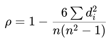
Where:

• di​ = the difference between the ranks of each observation
• n = the number of observations

Kendall tau coefficient (τ)

Kendall tau coefficient also measures monotonic relationships using ranks but is based on the number of concordant and discordant pairs. It’s more robust in the presence of ties and small samples.

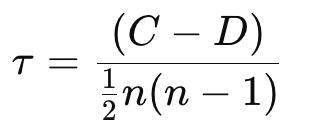
Where:

• C = number of concordant pairs (pairs that are ranked in the same order in both variables)
• D = number of discordant pairs (pairs that are ranked in different orders)
• n = number of observations

Conclusion

I hope you found this article helpful. As you have seen, correlation is a fundamental data analysis tool for understanding relationships between variables. 

Make sure you take our courses to keep learning. I recommend our Statistics Fundamentals in Python skill track or our Introduction to Statistics in R course as great next steps.