Gaussian Distribution: A Comprehensive Guide

Few concepts are as fundamental and widely applicable in statistics and data science as the Gaussian distribution. Also known as the normal distribution, this mathematical model underpins countless statistical methods and data analysis techniques.

This comprehensive guide unpacks the concept of Gaussian distributions, exploring their properties, applications, and significance in modern data analysis. We'll examine why they're so prevalent in natural phenomena and how they're used in various fields, from finance to manufacturing.

If you're new to statistics or want to brush up on the basics, our Introduction to Statistics course provides an excellent foundation. For those ready to apply these concepts in specific programming languages, our Statistical Thinking in Python (Part 1) and Statistics Fundamentals with R courses will help you appreciate the many ways in which the Gaussian distribution appears in descriptive and inferential statistics. 

What is a Gaussian Distribution?

A Gaussian distribution, also known as a normal distribution, is a continuous probability distribution characterized by its bell-shaped curve. It is defined by two parameters:

1. μ (mu): The mean or expected value of the distribution
2. σ (sigma): The standard deviation, which measures the spread of the distribution

The probability density function (PDF) of a Gaussian distribution is given by:

Where:

• x is the variable
• e is Euler's number (approximately 2.71828)
• π (pi) is the mathematical constant pi (approximately 3.14159)

Visualizing the Gaussian distribution

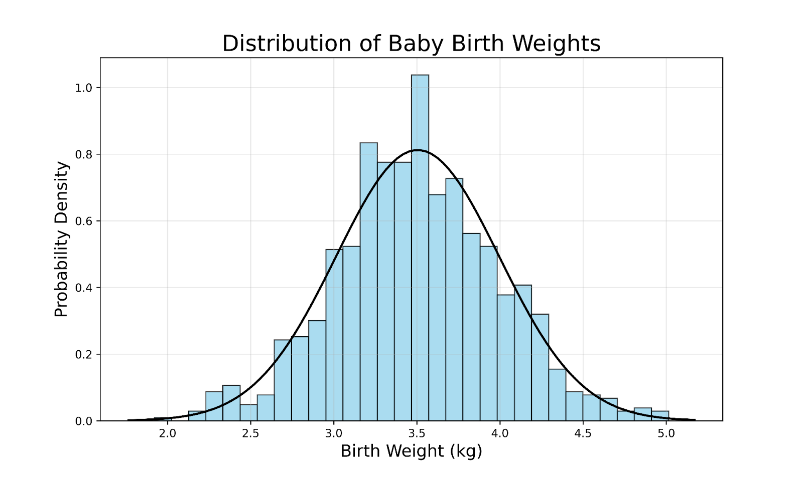
To illustrate the concept of a Gaussian distribution, consider the distribution of birth weights for full-term babies in a large population:

Some key observations from this graph include:

• Most babies' birth weights cluster around an average value (the peak of the curve).
• Fewer babies have birth weights that deviate significantly from this average.
• Very few babies have extreme birth weights (very high or very low).

The central limit theorem

The prevalence of Gaussian distributions in nature and statistics can be explained by the central limit theorem (CLT). The CLT states that the distribution of sample means approaches a normal distribution as the sample size increases (e.g., n ≥ 30) regardless of the underlying population's distribution.

One key aspect of the CLT is that this convergence to a normal distribution happens relatively quickly as the sample size increases. For most practical purposes, even moderately sized samples (e.g., n ≥ 30) are enough for the sample means to approximate a normal distribution. This is true even if the population itself is skewed.

The standard Gaussian distribution

Within the class of Gaussian distributions, there's a special case known as the standard Gaussian distribution, also known more commonly as the standard normal distribution. This is a Gaussian distribution where:

• The mean (μ) is exactly 0.
• The standard deviation (σ) is exactly 1.

The probability density function of a standard Gaussian distribution is given by the following formula. 

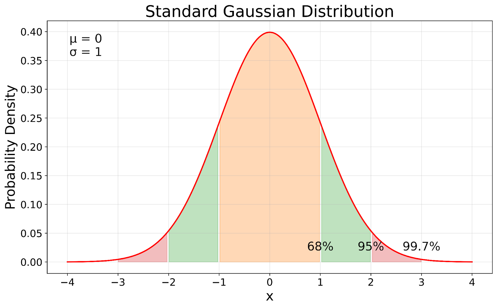
Notice that the formula for the standard Gaussian probability density function simplifies from the general form because of the specific values assigned to the mean and standard deviation. Now, let’s visualize the standard Gaussian distribution.

Standard Gaussian distribution. Image by Author

The standard Gaussian distribution, shown in our visualization, serves as a reference point in statistics. In our visual, you can see how the standard Gaussian is a standardized version of any Gaussian distribution. The process of standardization shifts the mean to 0 and scales the standard deviation to 1 while preserving the fundamental properties of the distribution.

Properties of Gaussian Distributions

Let’s now look at some of the properties of Gaussian distributions.

Symmetry and the bell curve

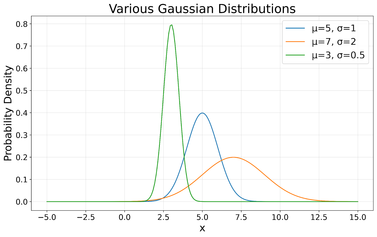
The hallmark of a Gaussian distribution is its symmetrical bell shape. This symmetry means that data is equally likely to fall above or below the mean, which is particularly useful in predicting probabilities and making inferences about data. As shown in the following visualization, all Gaussian distributions maintain this characteristic bell shape, regardless of their mean or standard deviation.

Gaussian distributions visualized. Image by Author

Mean, median, and mode alignment

In a perfect Gaussian distribution, the mean (average), median (middle value), and mode (most frequent value) are all the same. This alignment provides a clear indication of the data's central tendency, which is valuable for summarizing datasets. In our visualization, you can see how the peak of each curve represents this central point.

Standard deviation and data spread

The standard deviation in a Gaussian distribution tells us how spread out the data is from the mean. It follows a predictable pattern:

• About 68% of the data falls within one standard deviation of the mean.
• About 95% falls within two standard deviations.
• About 99.7% falls within three standard deviations.

This rule, known as the 68-95-99.7 rule, applies to all Gaussian distributions, regardless of their mean or standard deviation. 

Practical Applications of Gaussian Distributions

Gaussian distributions are more than just a theoretical concept – they have wide-ranging applications in various fields. 

Statistical inference and hypothesis testing

Many statistical tests, such as t-tests and ANOVA, assume that data is normally distributed. These tests help researchers determine if there are significant differences between groups or if observed effects are likely due to chance. The assumption of normality allows researchers to calculate p-values and confidence intervals, providing a framework for drawing conclusions from data and making informed decisions. 

The assumption of normality is so important that resampling techniques like bootstrapping have been developed to generate normally distributed resampling distributions from non-normal data, making it easier to construct confidence intervals and perform other statistical analyses. Our tutorial on hypothesis testing showcases how to conduct these tests under various scenarios including situations where data are normally distributed.

Machine learning algorithms

Many machine learning techniques rely on assumptions of normality, making Gaussian distributions fundamental to their operation and interpretation. In linear regression, for instance, we typically want to see the y values (dependent variable) follow a normal distribution to have confidence in our estimates. Additionally, we aim for the residuals (the differences between observed and predicted values) to have a normal distribution. These normality assumptions underpin the statistical tests used to assess the model's reliability and the confidence intervals for its predictions.

Also, machine learning scientists might prefer working with data that follows a Gaussian distribution for reasons of computational efficiency. A Gaussian distribution can indirectly contribute to computational efficiency in certain algorithms, especially those that assume or rely on data being normally distributed.

• Efficient Parameter Estimation: In a Gaussian distribution, the mean and variance are sufficient statistics, meaning they fully describe the distribution. This reduces the need for complex modeling of higher moments, speeding up parameter estimation.
• Algorithm Convergence: Algorithms like gradient descent, used for optimization in machine learning, converge faster if the data is normally distributed. 
• Reduced Computational Complexity in Some Algorithms: Algorithms like Gaussian naive Bayes are designed specifically for normally distributed data and can be computationally efficient when the assumption holds.