Simple Linear Regression: Everything You Need to Know

Every story starts somewhere, and for the data analyst or data scientist, the start of the story is often simple linear regression. Indeed, simple linear regression is perhaps the most foundational model of all. So, if you are serious about becoming a data analyst or data scientist, simple linear regression (and regressions generally) are an absolute must-know.

The reason regression is worth learning is not only because it is invaluable technique to answer pressing questions in practically every field, but it also opens the door for a deeper understanding of a huge variety of other things, like hypothesis testing, causal inference, and forecasting. So take our Introduction to Regression in R course and our Introduction to Regression with statsmodels in Python course today.

What is Simple Linear Regression? 

Simple linear regression is a linear regression with one independent variable, also called the explanatory variable, and one dependent variable, also called the response variable. In simple linear regression, the dependent variable is continuous. 

Ordinary least squares estimator 

The most common way to do simple linear regression is through ordinary least squares (OLS) estimation. Because OLS is by far the most common method, the “ordinary least squares” part is often implied when we talk about simple linear regression.

Ordinary least squares works by minimizing the sum of the squared differences between the observed values (the actual data points) and the predicted values from the regression line. These differences are called residuals, and squaring them ensures that both positive and negative residuals are treated equally. 

How Simple Linear Regression is Used

Simple linear regression helps make predictions and understand relationships between one independent variable and one dependent variable. For example, you might want to know how a tree’s height (independent variable) affects the number of leaves it has (dependent variable). By collecting data and fitting a simple linear regression model, you could predict the number of leaves based on the tree's height. This is the ‘making predictions’ part. But this approach also reveals how much the number of leaves changes, on average, as the tree grows taller, which is how simple linear regression is also used to understand relationships.  

Simple linear regression equation

Let's take a look at the simple linear regression equation. We can start by first looking at the slope-intercept form of a straight line using notation that is common in geometry or algebra textbooks. That is, we will start at the beginning.

Here

• m is the slope of the line
• b is the intercept

In the context of data science, you are more likely to see this equation instead: 

Where

• b0 is the y-intercept 
• b1 is the slope

The notation involving b0 and b1 helps us understand that we are looking at a situation where we are making a prediction on y, which is why we call it ŷ, or y-hat, since we don’t expect our regression line will actually go through all the points. 

The following visualization shows the conceptual difference between the slope-intercept form of the line, on the left, and the regression equation, on the right. In the language of linear algebra, we would say that the system of linear equations is overdetermined, meaning there are the more equations (thirty or so) than there are unknowns (two), so we don’t expect to find a solution.

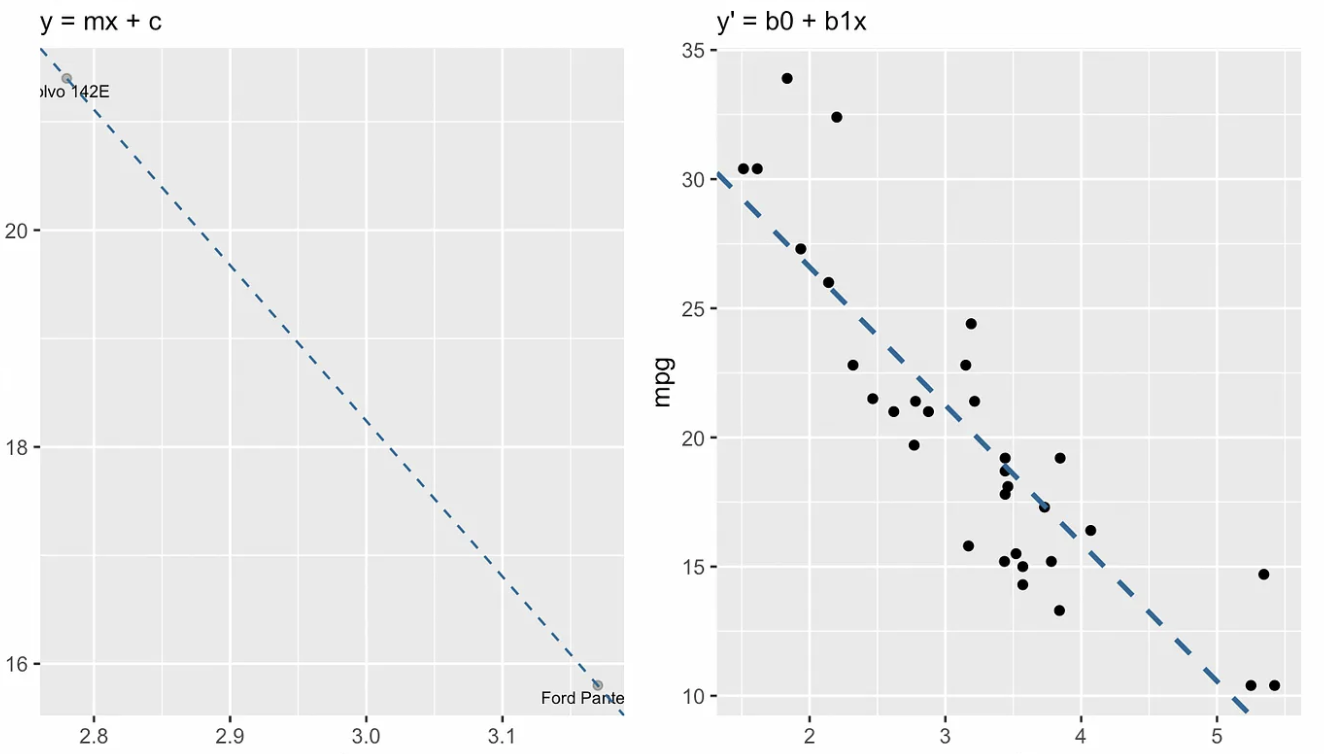Slope-intercept form vs. simple linear regression equation. Image by Author

Simple linear regression model coefficients

If we were using only the slope-intercept equation, we would find the values of m (slope) and b (y-intercept) by first calculating the slope as ‘rise over run,’ by which we mean measuring the change in y over the change in x between two points on the line. Then, once we have found the slope, we would find the y-intercept b by substituting the coordinates of one point on the line into the equation and solving for b. This final step gives you the point where the line crosses the y-axis.

This doesn’t work in regression because there is no line that goes through all the points, which is why we are finding instead the line of best fit. Fortunately, there are neat, closed-form equations to find the slope and intercept. 

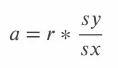
The slope can be calculated by multiplying the correlation r by the quotient of standard deviation of y over standard deviation of x. This makes intuitive sense because we are essentially converting the correlation coefficient back into units of the original variables. In the below equation, a refers to the slope and sy and sx refer to the standard deviation of y and the standard deviation of x, respectively.

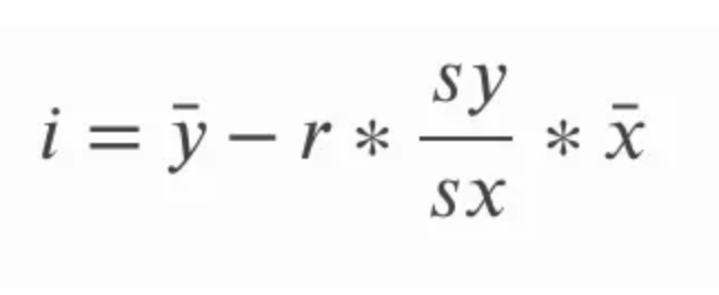
The intercept of the line of best fit for simple linear regression can be calculated after we calculate the slope. We do this by subtracting the product of the slope and the mean of x from the mean of y. In the equation below, i refers to y-intercept and the straight line over the x and y values is a way of referring to the mean of x and y respectively; we refer to these terms as x-bar and y-bar.

In the interest of being thorough, we can explore alternative ways of writing these equations. Remember that the standard deviation is the same as the square root of the variance, so instead of referring to the standard deviation of y and the standard deviation of x, we could also refer to the square root of the variance of y and the square root of the variance of x. The variance itself, we remember, is the average of the sum of squares. 

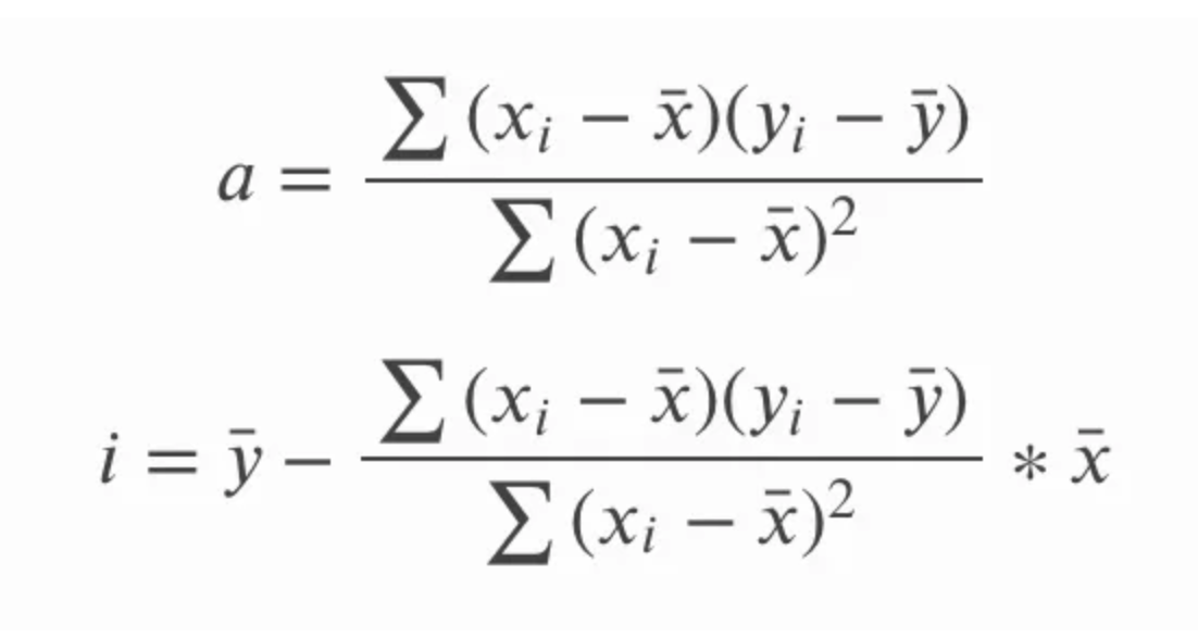
In the above equation for the slope, a, we could also write the sy and sx in terms of the standard deviation, and we could also write out the longer form equation for the correlation r. We could then cross-multiply and simplify the equation by removing common terms and end up with the following set of equations for the slope and intercept. The point here is less about showing how one equation turns into the other and more about stressing that both equations are the same since you might see one or the other. 

Another interesting consequence here is that the simple linear regression line will go through the central point, which is the mean of x and mean of y. In other words, the simple linear regression intersects at the average of both the independent and dependent variables, regardless of the distribution of data points, which helps gives the simple linear regression its sort of ‘balancing’ property.

Additional ways to find the simple linear regression model coefficients 

We saw how to find the simple linear regression model coefficients using neat equations. Here, we will look in more detail at some other methods involving linear algebra and calculus. Programming environments, in particular, solve through more advanced techniques because these techniques are faster and more precise (the thing about squaring to find the variance may reduce precision).

• Linear Algebra: There are some techniques from linear algebra to find the coefficients of a simple linear regression. We can find the coefficients in a simple linear regression model by solving what is known as the normal equation. The normal equation is interesting but a little inadvisable with large datasets because it involves matrix inversion, which can be expensive. Another linear algebra technique is to solve through QR decomposition, which doesn't have matrix inversion and is also known to be numerically stable.
• Calculus: We could find the slope and intercept of a simple linear regression model by taking the partial derivatives of the sum of squared errors (SSE) with respect to the slope and intercept and setting them equal to zero to solve for the coefficients. That’s one option. Another option with ties to calculus is gradient descent, which is an iterative optimization technique that can be used to minimize the SSE and find the slope and intercept. Gradient descent is closely tied to calculus because it relies on the gradient, which is the vector of partial derivatives.

Simple linear regression model assumptions

Let’s take a look now at the main simple linear regression model assumptions. If these assumptions are violated, we might want to consider a different approach. The first three, in particular, are strong assumptions and shouldn’t be ignored.

1. Linearity: The relationship between the independent and dependent variables must be linear. If the relationship is non-linear, the model won’t capture it well.
2. Independence of Errors: Residuals should be independent of each other. This means there should be no patterns or correlations between the residuals. This is something to watch for closely in time-ordered data.
3. Homoscedasticity: The residuals should have constant variance across all values of the independent variable. If the variance changes (heteroscedasticity), predictions in certain ranges of x may become less accurate.
4. Normality of Residuals: Residuals should ideally follow a normal, or Gaussian distribution. This is important for statistical testing, and asserting levels of confidence in our estimate. It’s less critical for making predictions. 

Simple linear regression model evaluation

Let’s say we have created a simple linear regression model. How do we know if it was a good fit? To answer this, we can look at diagnostic plots and model statistics. 

Simple linear regression diagnostic plots

Diagnostic plots help us see if a simple linear regression model fits well and doesn’t violate our assumptions. Any patterns or deviations in these plots suggest model issues that need attention or information that wasn’t captured. One diagnostic plot that is unique to simple linear regression is the x values versus residuals plot, as you can see below. Additional plots include the Q-Q plot, scale-location plot, observation number vs. cook’s distance, and others. 

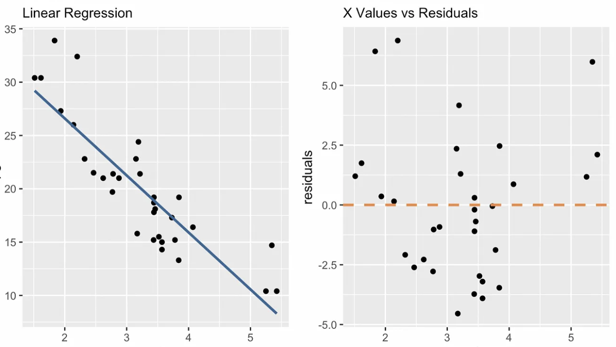x values vs. residuals diagnostic plot. Image by Author

Simple linear regression model statistics

Model statistics like R-squared and Adjusted R-squared quantify how well the independent variable explains the variance in the dependent variable. The F-statistic tests the overall significance of the model, and p-values for coefficients tell us about the impact of individual predictors. 

How to Interpret a Simple Linear Regression Model

When interpreting the results of simple linear regression, we should be careful to be exact in how we talk about the relationship between the independent variable and the dependent variable.

How to interpret the slope and the intercept

In particular, we should be careful how we talk about the two key components: the slope and the intercept.

• The intercept tells you where the regression line crosses the y-axis. In practical terms, it represents the value of the dependent variable when the independent variable is zero. It’s important to know that the intercept is not always interpretable. In our earlier example with trees, our model might have predicted a certain number of leaves for trees with a height of zero. It wouldn’t have made sense to try to interpret the intercept in this context. 
• The slope indicates how much the dependent variable is expected to change with a one-unit increase in the independent variable. A positive slope suggests a positive relationship, where the dependent variable increases as the independent variable increases. A negative slope indicates the opposite.

One important thing to consider is that correlation does not equal causation. Analysts who are familiar with this concept might still goof up when interpreting a simple linear regression because they are unpracticed with the words to use. You would not say that tree height causes more leaves, but rather you could say that a one-unit increase in tree height is associated with an increase in a certain number of leaves. 

Another important consideration is that extrapolating beyond the range of the data might not yield reliable predictions. A simple linear regression model that predicts the number of leaves from the height of the tree might not be very accurate for very short or very tall trees, especially if short or tall trees were not considered in the creation of our model. 

How to think about transformations

Linear models are called linear models because they are linear in their functional form. Specifically, in simple linear regression, the relationship between the response variable y and the predictor variable x is modeled as a linear combination of the predictor and a constant. That said, you might be surprised by what you can do with a simple linear regression. While the model assumes a straight-line relationship between variables, you can introduce transformations to capture non-linear relationships.

For example, consider the non-linear relationship representing the growth of ancestors by generation where the number of ancestors seems to grow exponentially with each generation: two parents, four grandparents, eight great-grandparents, and so on. You would not expect a linear model to capture exponential growth, but by predicting the log(y) instead of y, you linearize the relationship. 

Thinking further, however, you realize that there isn’t exponential growth in ancestors because of something called pedigree collapse, which is where the growth rate slows dramatically over time because distant ancestors appear in multiple places in the family tree. For this reason, taking the log(y) may have over-amplified our model. Now, to soften this, we can create a new variable that is a square root transformation on x and use this as our predictor instead. Now, I’m not saying any of this model is correct, or trying to fully interpret it, but I am trying to show how log(y) and square root of x are non-linear transformations that enter the equation linearly with respect to the coefficients, so we still have a simple linear regression.  

Simple Linear Regression in R and Python

Let’s consider simple linear regression in R and Python.

R programming

R is one great option for simple linear regression.

Manually calculating the slope and intercept

We can find the coefficients ourselves by calculating the mean and standard deviation of our variables. 

# Manually calculate the slope and intercept in R

# Sample data
X <- c(1, 2, 3, 4, 5)
y <- c(2, 4, 5, 4, 5)

# Calculate means
mean_X <- mean(X)
mean_y <- mean(y)

# Calculate standard deviations
sd_X <- sd(X)
sd_y <- sd(y)

# Calculate correlation
correlation <- cor(X, y)

# Calculate slope (b1) using the formula: b1 = (correlation * sd_y) / sd_X
slope <- (correlation * sd_y) / sd_X

# Calculate intercept (b0) using the formula: b0 = mean_y - slope * mean_X
intercept <- mean_y - slope * mean_X

# Print the slope and intercept
cat("Slope (b1):", slope, "\n")
cat("Intercept (b0):", intercept, "\n")

# Use the manually calculated coefficients to predict y values
y_pred <- intercept + slope * X
cat("Predicted values:", y_pred, "\n")

Using the lm() function

In R, we can create a regression using the lm() function, which we can access without needing to use any libraries. 

# Fit the model 
model <- lm(y ~ X) 

# Print the summary of the regression 
summary(model)

Python

Python is another great option for simple linear regression. 

Manually calculating the slope and intercept

Here we find the mean and standard deviation for each variable. 

import numpy as np

# Sample data
X = np.array([1, 2, 3, 4, 5])
y = np.array([2, 4, 5, 4, 5])

# Calculate means
mean_X = np.mean(X)
mean_y = np.mean(y)

# Calculate standard deviations
sd_X = np.std(X, ddof=1)
sd_y = np.std(y, ddof=1)

# Calculate correlation
correlation = np.corrcoef(X, y)[0, 1]

# Calculate slope (b1) using the formula: b1 = (correlation * sd_y) / sd_X
slope = (correlation * sd_y) / sd_X

# Calculate intercept (b0) using the formula: b0 = mean_y - slope * mean_X
intercept = mean_y - slope * mean_X

# Print the slope and intercept
print(f"Slope (b1): {slope}")
print(f"Intercept (b0): {intercept}")

# Use the manually calculated coefficients to predict y values
y_pred = intercept + slope * X

print(f"Predicted values: {y_pred}")

Using statsmodels

statsmodels is one option for simple linear regression.

import statsmodels.api as sm

# Adding a constant for the intercept
X = sm.add_constant(X)

# Fit the model
model = sm.OLS(y, X)
results = model.fit()

# Print the summary of the regression
print(results.summary())

Simple Linear Regression, t-test, and ANOVA

Simple linear regression is used in hypothesis testing and is central in t-tests, and analysis of variance (ANOVA). 

Simple linear regression and t-test

A t-test is often used to determine whether the slope of the regression line is significantly different from zero. This test helps us understand whether the independent variable has a statistically significant effect. Basically, we formulate a null hypothesis stating that the slope of the regression line is equal to zero, meaning that there is no linear relationship, and the t-test evaluates this. Simple linear regression ties in here because a simple linear regression with a binary independent variable is the same as a difference in means, as we see in a t-test.

Simple linear regression and ANOVA

Analysis of variance (ANOVA) is a statistical method used to assess the overall fit of the model and to determine if the independent variable explains a significant portion of the variance in the dependent variable. What we do is partition the total variance of the dependent variable into two components: the variance explained by the regression model (between groups) and the variance due to residuals or error (within groups). The F-test in ANOVA essentially tests whether the regression model, as a whole, fits the data better than a model with no predictors. For instance, in our tree height and leaf count example, ANOVA would help determine if incorporating tree height significantly improves our ability to predict the number of leaves.

Alternatives to OLS Simple Linear Regression 

We said that ordinary least squares is by far the most common estimator in simple linear regression, and we have focused on OLS in this article. However, we should consider that the ordinary least squares estimator is sensitive to, or not robust against, outliers. So adding a highly influential or high leverage data point could dramatically change the slope and intercept of the line.  

For this reason, non-parametric options exist. The following visualization shows ordinary least squares with three non-parametric alternatives: median absolute deviation (MAD), least median squares (LMS), and Theil-Sen. Notice that the slope and intercept are different for each estimator. If we were to add a highly influential point at, say, coordinates x = 7 and y = 70, then the ordinary least squares regression line would change the most.

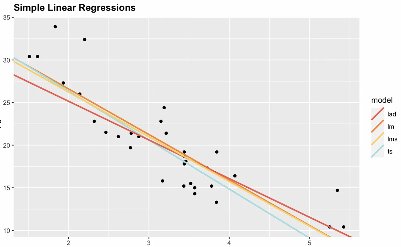Four simple linear regression options. Image by Author

Final Thoughts

Simple linear regression is the starting point for understanding more complex relationships in data. To help, DataCamp offers tutorials so you can keep practicing, including our Essentials of Linear Regression in Python tutorial, How to Do Linear Regression in R tutorial, and the Linear Regression in Excel: A Comprehensive Guide For Beginners tutorial. These resources will guide you through using different tools to perform linear regression and understand its applications. Finally, if you are ready to expand your skills, look into our Multiple Linear Regression in R: Tutorial With Examples, which covers more complex models involving multiple predictors.