R-Squared Explained: How Well Does Your Regression Model Fit?

At its core, R-squared explains the proportion of variance in the dependent variable that can be attributed to the independent variable (or variables). We can think of it as a measure of how well our model captures the story in the data, and how much is left as unexplained noise. Its simplicity and direct interpretation make it widespread in linear regression diagnostics, especially in simple and multiple linear regression.

In this article, we’ll discuss the meaning, calculation, interpretation, and common pitfalls surrounding R-squared, so we can use it with both confidence and care. In addition, we’ll take a look at some examples of code snippets for calculating R-squared in R and Python.

What Is R-Squared?

R-squared, denoted as R^², is a statistical measure of goodness of fit in regression models. It tells us how much of the variation in the dependent variable can be explained by the model.

The value of R-squared lies between 0 and 1:

• R^² = 0 means the model explains none of the variability;
• R^² = 1 means the model explains all of it.

While the concept is straightforward, its interpretation requires a nuanced approach, especially when moving from theory to practice.

How to Calculate R-Squared

There are several mathematically equivalent ways to compute R-squared, each offering a different insight on what “fit” really means, depending on the context—simple regression, multiple regression, matrix algebra, or Bayesian modeling. Let’s explore the most frequently used of these approaches.

1. Using residual sum of squares and total sum of squares

This is the most standard and widely used formula:

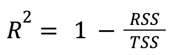
where:

• RSS is the residual sum of squares, measuring the unexplained variation by the model,
• TSS is the total sum of squares, measuring the total variation in the data.

In other words, R-squared represents the fraction of the total variation that the model accounts for. 

This approach highlights how much better the regression model performs compared to simply predicting the mean of the response.

2. Using explained sum of squares and total sum of squares

R-squared can also be expressed directly in terms of explained variance:

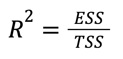
where:

• ESS is the explained sum of squares, measuring how much of the variance is captured by the model,
• TSS is the total sum of squares, measuring the total variation in the data.

We can see that this version emphasizes how much of the total variation in the outcome is captured by the model’s predictions. In other words, the focus here is shifted from what we failed to explain (RSS) to what we did (ESS), providing a more optimistic framing.

For a deep dive into the three components of the sum of squares, read Understanding Sum of Squares: A Guide to SST, SSR, and SSE.

3. Using explained sum of squares and residual sum of squares

In the context of an ANOVA table, R-squared naturally emerges from the decomposition of total variability: 

where:

• ESS is the explained sum of squares, measuring how much of the variance is captured by the model,
• RSS is the residual sum of squares, measuring the unexplained variation by the model.

This formulation shows how much of the total variance is picked up by the model, and how much is left unexplained.

This perspective is a little bit unique because it ties R-squared to hypothesis testing. This is because the ratio of ESS to RSS is used to compute the F-statistic, making R-squared a big part of significance testing in ANOVA-style reporting.

4. Using correlation coefficient in simple linear regression

The last three methods were all algebraically equivalent formulas derived from regression decomposition. Now, here is a new perspective:

In simple linear regression with just one predictor, R-squared has a shortcut:

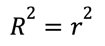
where

• r is the Pearson correlation coefficient between x and y.

This formula shows how a strong linear relationship between two variables translates directly into a high R-squared. 

To understand the underlying theory behind simple linear regression, go through Simple Linear Regression: Everything You Need to Know.

5. Using mean squared error and the variance of the outcome

R-squared can be calculated as a normalized measure of model error: 

where:

• MSE is the mean squared error of the model,
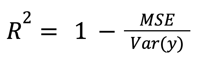
• Var(y) is the variance of the true outcome.

This framing is especially relevant when comparing models across different scales or units, because it normalizes model error by overall data spread.

6. Using the variance of predicted values

Assuming the residuals are uncorrelated with the predictions, R-squared can also be interpreted as the fraction of variance captured by the model:

where:

• Var(ŷ) is the variance of the model’s predictions,
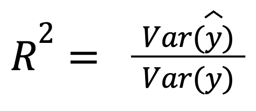
• Var(y) is the variance of the true outcome.

This version highlights how well the predictions themselves reflect the spread of the actual data.

Interpreting R-Squared

As we’ve mentioned earlier, R-squared is easy to calculate but a bit trickier to interpret meaningfully.

• A high R-squared means the model explains a large portion of the variance. However, it doesn’t mean our model is necessarily correct or useful.
• A low R-squared means little variance is explained by the model. This isn’t always bad, especially in social sciences or noisy data, where a low R-squared is often expected.

It’s important to remember that R-squared measures correlation, but it doesn’t measure causality. Just because our predictors explain the outcome doesn't mean they cause it, because correlation still doesn’t mean causation. Besides, R-squared doesn’t indicate whether predictions are accurate.

Here are two useful resources on more advanced topics related to linear regression: 

• Variance Inflation Factor (VIF): Addressing Multicollinearity in Regression Analysis
• QR Decomposition in Machine Learning: A Detailed Guide

When to Use R-Squared

R-squared can be very helpful if used in the right situations. It’s appropriate for:

• Comparing models with the same number of predictors.
• Explaining how much variance in a dataset is accounted for by the model.

On the other hand, R-squared can be misleading in the following scenarios:

• Adding irrelevant predictors, which results in overfitting. In this case, R-squared always increases even if the predictive performance of the model doesn't improve.
• Comparing models with different numbers of predictors, i.e., with different complexities. Here, adjusted R-squared is a better choice. I'll talk more about adjusted R-squared later on.

R-Squared Examples in R and Python

Let’s now illustrate the concept of R-squared in R and Python using the Fish Market Kaggle dataset. In both programming languages, we'll build two models:

• Model 1: Predict fish weight using four predictors.
• Model 2: Add a random, irrelevant predictor.

R example

Let's start with R.

Model 1

# Load data
fish <- read.csv("Fish.csv")

# Model 1
model1 <- lm(Weight ~ Length1 + Length2 + Height + Width, data=fish)
summary(model1)$r.squared

Output:

[1] 0.8673

Model 2

# Model 2 with an irrelevant predictor
fish$random_noise <- rnorm(nrow(fish))
model2 <- lm(Weight ~ Length1 + Length2 + Height + Width + random_noise, data=fish)
summary(model2)$r.squared

Output:

[1] 0.8679

As we can see, R-squared increases slightly after adding an irrelevant predictor (Model 2). However, that doesn't mean the model got better. After all, we just added random noise.

For further reading on the topic, see the following tutorials:

• How to Do Linear Regression in R
• Multiple Linear Regression in R: Tutorial With Examples

And remember to enroll in our designated course:

• Introduction to Regression in R course

Python example

Now, let's try in Python.

Model 1

import pandas as pd
import statsmodels.api as sm
import numpy as np

# Load data
fish = pd.read_csv('Fish.csv')
X1 = fish[['Length1', 'Length2', 'Height', 'Width']]
y = fish['Weight']

# Model 1
X1 = sm.add_constant(X1)
model1 = sm.OLS(y, X1).fit()
print(model1.rsquared)

Output:

0.8673

Model 2

# Model 2 with an irrelevant predictor
fish['random_noise'] = np.random.randn(len(fish))
X2 = fish[['Length1', 'Length2', 'Height', 'Width', 'random_noise']]
X2 = sm.add_constant(X2)
model2 = sm.OLS(y, X2).fit()
print(model2.rsquared)

Output:

0.8679

Again, we observe a slight increase in the R-squared value, but this is just capturing random noise.

To keep learning, enroll in our courses:

• Introduction to Regression with statsmodels in Python and
• Intermediate Regression with statsmodels in Python

R-Squared vs. Related Metrics

Now we’ll briefly compare R-squared with two related metrics: adjusted R-squared and predicted R-squared.

R-squared vs. adjusted R-squared

Unlike R-squared, adjusted R-squared accounts for the number of predictors. In particular, it penalizes the model for including unnecessary predictors:

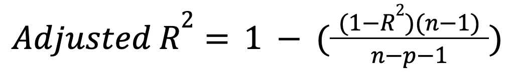
where:

• n is the number of observations,
• p is the number of predictors.

This metric only increases if a new predictor actually improves the model meaningfully, and can decrease in the opposite case. Read our tutorial to learn more about this important extension: Adjusted R-Squared: A Clear Explanation with Examples.

R-squared vs. predicted R-squared

While regular R-squared shows how well the model performs on the training data, predicted R-squared tells us how well it does on new, unseen data. Hence, this metric evaluates the model’s generalization ability.

Predicted R-squared is calculated using cross-validation or by holding out part of the training data for further testing. It can be significantly lower than regular R-squared if the model is overfitted. Therefore, a scenario where we get a high value of regular R-squared but a low value of predicted R-squared can most likely indicate model overfitting.

Common Misconceptions About R-Squared

Let’s take a look at some popular myths about R-squared, along with the true state of things: 

• “A high R-squared always means a good model.” This is not necessarily true. R-squared can be high for an overfitted model or one built on spurious correlations. Naturally, in both cases, the model can’t be referred to as good.
• “R-squared measures predictive power.” In reality, it only measures model fit on the training data and says nothing about unseen data. To evaluate future model performance, we need other metrics like the above-discussed predicted R-squared.
• “We should always aim for a high R-squared.” Well, not always. It depends on the domain, as well as on the data quality itself. As we’ve mentioned earlier in this article, for social sciences like psychology or history, the value of R-squared can be very low (0.1 or even less) and still meaningful. The same regards noisy data, where a low value of R-squared is highly expected.

Conclusion

To sum up, we learned what R-squared is, how to calculate this metric (both mathematically and in R and Python), when to use and when to avoid it, and how to interpret the results. Besides, we touched on two related metrics and some widespread misconceptions about R-squared. 

In a nutshell, R-squared is a useful, intuitive, and straightforward measure of a regression model fit. It’s a great starting point for model evaluation, but it should be used wisely, interpreted alongside other metrics, and not be mistaken for the whole picture. This is especially true for multiple regression and model selection contexts.