Explainable AI - Understanding and Trusting Machine Learning Models

What Is Explainable AI (XAI)?

Explainable AI refers to a set of processes and methods that aim to provide a clear and human-understandable explanation for the decisions generated by AI and machine learning models.

Integrating an explainability layer into these models, Data Scientists and Machine Learning practitioners can create more trustworthy and transparent systems to assist a wide range of stakeholders such as developers, regulators, and end-users.

Building Trust Through Explainable AI

Here are some explainable AI principles that can contribute to building trust:

• Transparency. Ensuring stakeholders understand the models’ decision-making process.
• Fairness. Ensuring that the models’ decisions are fair for everyone, including people in protected groups (race, religion, gender, disability, ethnicity).
• Trust. Assessing the confidence level of human users using the AI system.
• Robustness. Being resilient to changes in input data or model parameters, maintaining consistent and reliable performance even when faced with uncertainty or unexpected situations.
• Privacy. Guaranteeing the protection of sensitive user information.
• Interpretability. Providing human-understandable explanations for their predictions and outcomes.

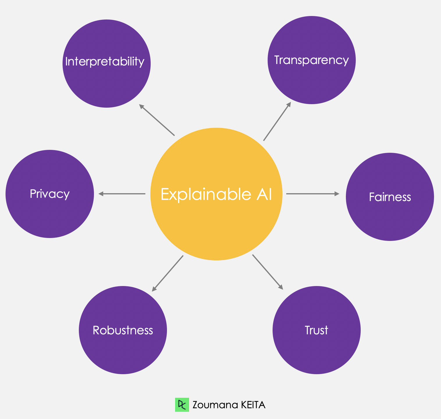
There are several benefits to implementing explainable AI. For decision-makers and other stakeholders, it offers a clear understanding of the rationale behind AI-driven decisions, enabling them to make better-informed choices. It also helps identify potential biases or errors in the models, leading to more accurate and fair outcomes.

Explainable AI Examples

There are two broad categories of model explainability: model-specific methods and model-agnostic methods. In this section, we will understand the difference between both, with a specific focus on the model-agnostic methods.

Both techniques can offer valuable insights into the inner working of machine learning models while ensuring that the models are effective and accountable.

To better illustrate these tools, we will use the diabetes dataset from Kaggle. First, we will build a simple classifier and then implement the explainability. The full source code is available in this DataLab workbook.

Build Classifier

A Random Forest classifier is built to predict diabetes outcomes using the diabetes dataset. The code is broken down into several steps: (1) import relevant libraries, (2) create training and testing datasets, (3) build the model, and (4) report the performance metrics through the classification report.

# Load useful libraries
from sklearn.model_selection import train_test_split
from sklearn.ensemble import RandomForestClassifier
from sklearn.model_selection import cross_val_score
from sklearn.metrics import classification_report

# Separate Features and Target Variables
X = diabetes_data.drop(columns='Outcome')
y = diabetes_data['Outcome']

# Create Train & Test Data
X_train, X_test, y_train, y_test = train_test_split(X, y,test_size=0.3,
                                                	stratify =y,
                                                	random_state = 13)

# Build the model
rf_clf = RandomForestClassifier(max_features=2, n_estimators =100 ,bootstrap = True)

rf_clf.fit(X_train, y_train)

# Make prediction on the testing data
y_pred = rf_clf.predict(X_test)

# Classification Report
print(classification_report(y_pred, y_test))

The last print statement generates the following report: 

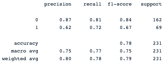
The random forest classifier provides a decent performance in predicting diabetes outcomes, with obvious room for improvement using different models.

Now, we can integrate the explainability layer into this model to provide more insights into its predictions. The next section will focus on the two broad categories of model explainability: model-specific methods and model-agnostic methods.

Our Classification in Machine Learning: An Introduction article helps you learn about classification in machine learning, looking at what it is, how it's used, and some examples of classification algorithms.

Model-agnostic methods

These methods can be applied to any machine learning model, regardless of its structure or type. They focus on analyzing the features’ input-output pair. This section will introduce and discuss LIME and SHAP, two widely-used surrogate models.

SHAP

It stands for SHapley Additive exPlanations. This method aims to explain the prediction of an instance/observation by computing the contribution of each feature to the prediction, and it can be installed using the following pip command.

!pip install shap

After the installation:

• The main shap library is imported.
• The TreeExplainer class is used to explain tree-based models, along with the initjs.
• shape.initjs() function initializes the JavaScript code required to display SHAP visualizations in a jupyter notebook environment.
• Finally, after instantiating the TreeExplainer class with the random forest classifier, the shape values are computed for each feature of each instance in the test dataset.

import shap
import matplotlib.pyplot as plt

# load JS visualization code to notebook
shap.initjs()

# Create the explainer
explainer = shap.TreeExplainer(rf_clf)

shap_values = explainer.shap_values(X_test)

SHAP offers an array of visualization tools for enhancing model interpretability, and the next section will discuss two of them: (1) variable importance with the summary plot, (2) summary plot of a specific target, and (3) dependence plot.

Variable Importance with Summary Plot

In this plot, features are ranked by their average SHAP values showing the most important features at the top and the least important ones at the bottom using the summary_plot() function. This helps to understand the impact of each feature on the model’s predictions.

print("Variable Importance Plot - Global Interpretation")
figure = plt.figure()
shap.summary_plot(shap_values, X_test)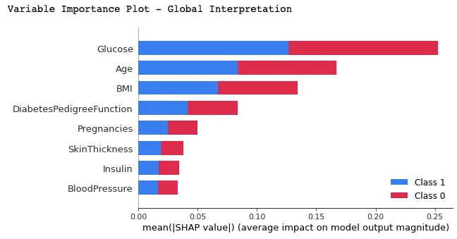

Below is the interpretation that can be made from the above graphic:

• We can observe that the red and blue colors occupy half of the horizontal rectangles for each class. This means that each feature has an equal impact on the classification of both diabetes (label=1) and non-diabetes (label=0) cases.
• However, Glucose, Age, and BMI are the first three features with the most predictive power.
• On the other hand, Pregnancies, SkinThicknes, Insulin, and BloodPressure do not contribute as much as the first three features.

Summary Plot on a Specific Label

Using this approach can provide a more granular overview of the impact of each feature on a specific outcome (label).

In the example below, shap_values[1] is used to represent the SHAP values for instances classified as label 1 (having diabetes).

shap.summary_plot(shap_values[1], X_test)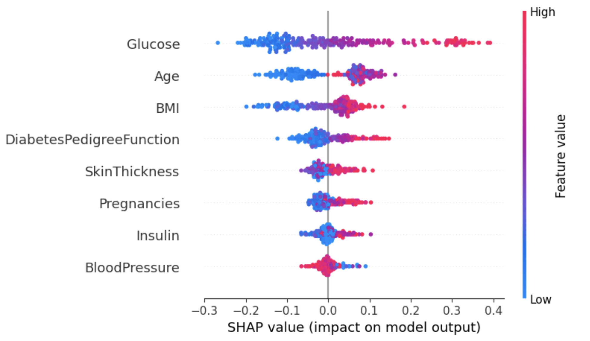

From the above graphic:

• Y-axis represents the features ranked by their average absolute SHAP values, similar to the graphic in image 2.
• X-axis represents SHAP values. Positive values for a given feature push the model’s prediction closer to the label being examined (label=1). In contrast, negative values push towards the opposite class (label=0).
• An individual with a high glucose (red dots) level is likely to be diagnosed with diabetes (positive outcome), while a low glucose level leads to not being diagnosed with diabetes.
• Similarly, aging patients are more likely to be diagnosed with diabetes. However, the model seems uncertain about the diagnosis for younger patients.

One way of dealing with this ambiguity for the Age attribute is using the dependence plot to gain more insights.

Dependence Plot

Unlike summary plots, dependence plots show the relationship between a specific feature and the predicted outcome for each instance within the data. This analysis is performed for multiple reasons and is not limited to gaining more granular information and validating the importance of the feature being analyzed by confirming or challenging the findings from the summary plots or other global feature importance measures. 

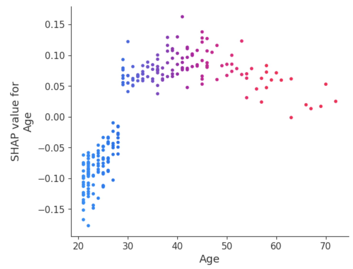
The dependence plot reveals that patients under 30 have a lower risk of being diagnosed with diabetes. In contrast, individuals over 30 face a higher likelihood of receiving a diabetes diagnosis.

LIME

Local Interpretable Model-agnostic Explanations (LIME for short). Instead of providing a global understanding of the model on the entire dataset, LIME focuses on explaining the model’s prediction for individual instances.

LIME explainer can be set up using two main steps: (1) import the lime module, and (2) fit the explainer using the training data and the targets. During this phase, the mode is set to classification, which corresponds to the task being performed.

# Import the LimeTabularExplainer module
from lime.lime_tabular import LimeTabularExplainer

# Get the class names
class_names = ['Has diabetes', 'No diabetes']

# Get the feature names
feature_names = list(X_train.columns)

# Fit the Explainer on the training data set using the LimeTabularExplainer
explainer = LimeTabularExplainer(X_train.values, feature_names =     
                                 feature_names,
                                 class_names = class_names, 
                                 mode = 'classification')

The code snippet below generates and displays a LIME explanation for the 8th instance in the test data using the random forest classifier and presenting the final feature contribution in a tabular format. 

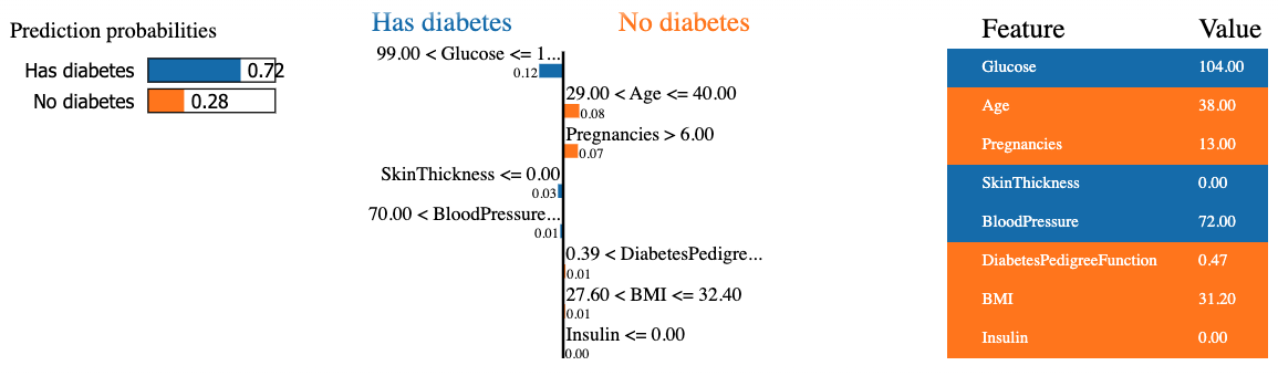
The result contains three main pieces of information from left to right: (1) the model’s predictions, (2) features contributions, and (3) the actual value for each feature.

We can observe that the eight patient is predicted to have diabetes with 72% confidence. The reasons that led the model to make this decision is because:

• The patient’s glucose level is more than 99.
• The blood pressure is more than 70.

Those values can be verified from the table on the right.

Model-specific methods

As opposed to model-agnostic methods, these methods can only be applied to a limited category of models. Some of those models include linear regression, decision trees, and neural network interpretability. Different technics such as DeepLIFT, Grad-CAM, or Integrated Gradients can be leveraged to explain deep-learning models.

When using a decision-tree model, a graphical tree can be generated with the plot_tree function from scikit-learn to explain the decision-making process of the model from top-to-bottom, and an illustration is given below.

The Deep Learning - A Tutorial for Data Scientists article will answer the most frequently asked questions about deep learning and explores various aspects of deep learning with real-life examples.

Let's train a decision tree classifier with specific hyperparameters like max_depth, and min_samples_leaf before generating the graphical tree.

from sklearn.tree import DecisionTreeClassifier, plot_tree
dt_clf = DecisionTreeClassifier(max_depth = 3, min_samples_leaf = 2)
dt_clf.fit(X_train, y_train)

# Predict on the test data and evaluate the model
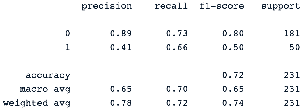
y_pred = dt_clf.predict(X_test)

print(classification_report(y_pred, y_test))

The previous print statement generates the following classification report of the model. 

And the model decision-making process can be visualized from the code below:

fig = plt.figure(figsize=(25,20))
_ = plot_tree(dt_clf,
               	feature_names = feature_names,
               	class_names = class_names,
               	filled=True)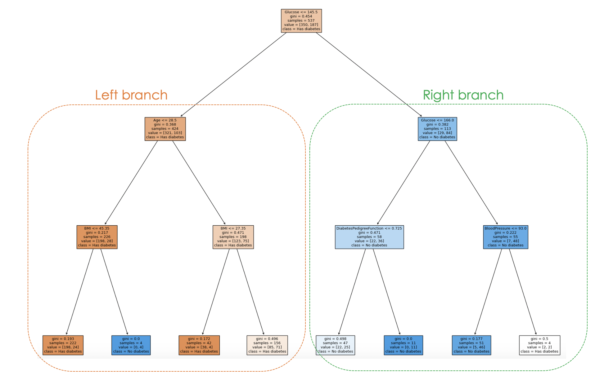

By examining the tree structure, one can trace the decision-making process for each sample, providing insights into the model's behavior and interpretability.

In the above plot, each node represents a decision or split based on a specific feature value. For each internal node, the plot shows the feature used for the split, the split criterion value, the Gini impurity, and the number of samples reaching that node.

In the leaf nodes, the majority class and the number of samples are displayed. Also, the colors in the nodes represent the majority class, with the intensity of the color indicating the proportion of the dominant class within that node. For instance, the orange nodes on the left branch correspond to the diabetes label, whereas the blue one corresponds to no diabetes.

Challenges of XAI and Future Perspectives

As AI technology continues to advance and become more sophisticated, understanding and interpreting the algorithms to discern how they produce outcomes is becoming increasingly challenging, allowing researchers to continue exploring new approaches and improving existing ones.

Many explainable AI models require simplifying the underlying model, leading to a loss of predictive performance. In addition, current explainability methods may not cover all the aspects of the decision-making process, which can limit the benefit of the explanation, especially when dealing with more complex models.

New research methods are focusing on enhancing explainable AI technics by developing more effective algorithms to address ethical issues while creating user-friendly explanations.

Finally, with the ongoing research, we are more likely to have more sophisticated methods that promote transparency, trustworthiness, and fairness.

Conclusion

This article has provided a good overview of what explainable AI is and some principles that contribute to building trust and can provide Data Scientists and other stakeholders with relevant skillsets to build trustworthy models to help make actionable decisions.

We also covered model-agnostic and model-specific methods with a special focus on the first one using LIME and SHAP. Furthermore, the challenges, limitations, and some areas of research have been highlighted about explainable AI.

To learn more about the ethics behind such technology, check out our Introduction to Data Ethics course, which covers principles of data ethics, its relationship with AI ethics, and its characteristics across the different stages of the data lifecycle.