Course
Case Study: Exploratory Data Analysis in R
4 hr
56.7K
The goal of this tutorial is to show you how you can gather data about H1B visas through web scraping with R. Next, you'll also learn how you can parse the JSON objects, and how you can store and manipulate the data so that you can do a basic exploratory data analysis (EDA) on the large data set of H1B filings.
Maybe you can learn how to best position yourself as a candidate or some new R code!
Last week, DataCamp's blog "Can Data Help Your H-1B Visa Application" presented you with some of the results of an analysis of H-1B data over the years. Now, it's time to get your hands dirty and analyze the data for yourself and to see what else you can find! Ted Kwartler will guide you through this with a series of R tutorials.
I have a friend at a Texas law firm that files H1B visas. The H1B is a non-immigrant visa in the United States of America that allows U.S. employers to employ foreign workers in specialty occupations temporarily. Apparently, getting accepted is extremely difficult because there is a limited visa supply versus thousands of applicants. Although that is anecdotal, I decided to explore the data myself in the hopes of helping qualified candidates know the US is a welcoming place!
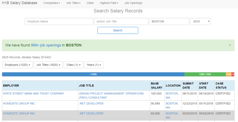
My DataCamp colleague pointed me to this site which is a simple website containing H1B data from 2012 to 2016. The site claims to have 2M H1B applications organized into a single table.I decided to programmatically gather this data (read: web scrape) because I was not about to copy/paste for the rest of my life! As you can see, the picture below shows a portion of the site showing Boston’s H1B data:
The libraries that this tutorial is going to make use of include jsonlite for parsing JSON objects, rvest which “harvests” HTML, pbapply, which is a personal favorite because it adds progress bars to the base apply functions, and data.table, which improves R’s performance on large data frames.
library(jsonlite)
library(rvest)
library(pbapply)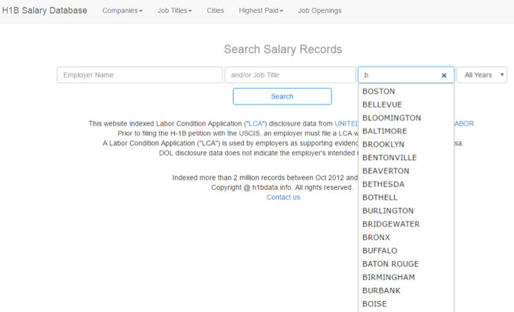
library(data.table)As you explore the site, you will realize the search form suggests prefill options. For instance, typing “B” into the city field will bring up a modal with suggestions shown below. The picture below shows the prefill options when I type “B”:
That means that you can use the prefill as an efficient way to query the site. Using Chrome, you can reload and then right click to “Inspect” the page, then navigate to “Network” in the developer panel and finally type in “B” on the page to load the modal.Exploring the network panel links, you will find a PHP query returning a JSON object of cities like this. The goal is first to gather all the suggested cities and then use that list to scrape a wide number of pages with H1B data. When you explore the previous URL, you will note that it ends in a letter. So, you can use paste0() with the URL base, http://h1bdata.info/cities.php?term=, and letters. The base is recycled for each value in letters. The letters object is a built-in R vector from “a” to “z”. The json.cities object is a vector of URLs, a to z, that contain all prefill suggestions as JSON.
json.cities<-paste0('http://h1bdata.info/cities.php?term=', letters)json.cities object is a vector of 26 links that have to be read by R. Using lapply() or pblapply() along with fromJSON, R will parse each of the JSON objects to create all.cities. You nest the result in unlist so the output is a simple string vector. With this code, you have all prefill cities organized into a vector that you can use to construct the actual webpages containing data.all.cities<-unlist(pblapply(json.cities,fromJSON))expand.grid().In the code below, you see that the city information is passed, all.cities, and then year using seq() from 2012 to 2016. The function creates 5000+ city year combinations. expand.grid() programmatically creates a Boston 2012, Boston 2013, Boston 2014, etc. because each city and each year represent a unique factor combination.
city.year<-expand.grid(city=all.cities,yr=seq(2012,2016))url_encode() function changes “Los Angeles” to Los%20Angeles to validate the address. You pass in the entire vector and url_encode() will work row-wise:
city.year$city<-urltools::url_encode(as.character(city.year$city))paste0() function again to concatenate the base URL to the city and state combinations in city.year. Check out an example link here.
all.urls<-paste0('http://h1bdata.info/index.php?em=&job=&city=', city.year[,1],'&year=', city.year[,2])Once you have gone through the previous steps, you can create a custom function called main to collect the data from each page.It is a simple workflow using functions from rvest. First, a URL is accepted and read_html() parses the page contents. Next, the page’s single html_table is selected from all other HTML information. The main function converts the x object to a data.table so it can be stored efficiently in memory. Finally, before closing out main, you can add a Sys.sleep so you won’t be considered a DDOS attack.
main<-function(url.x){
  x<-read_html(url.x)
  x<-html_table(x)
  x<-data.table(x[[1]])
  return(x)
  Sys.sleep(5)
}
Let’s go get that data! I like having the progress bar pblapply() so I can keep track of the scraping progress.
You simply pass all.urls and the main function in the pblapply() function. Immediately, R gets to work loading a page, collecting the table and holding a data.table in memory for that page. Each URL is collected in turn and held in memory.
all.h1b<-pblapply(all.urls, main)Phew! That took hours! At this point all.h1b is a list of data tables, one per page. To unify the list into a single data table, you can use rbindlist. This is similar to do.call(rbind, all.h1b) but is much faster.
all.h1b<-rbindlist(all.h1b)
Finally save the data so you don’t have to do that again. Lucky for you, I saved a copy here.
write.csv(all.h1b,'h1b_data.csv', row.names=F)
Even though you scraped the data, some additional steps are needed to get it into a manageable format.
You use lubridate to help organize dates. You also make use of stringr, which provides wrappers for string manipulation.
library(lubridate)
library(stringr)
Although this is a personal preference, I like to use scipen=999. It’s not mandatory but it gets rid of scientific notation.
options(scipen=999)It turns out the web scrape captured 1.8M of the 2M H1B records. In my opinion, 1.8M is good enough. So let’s load the data using fread(): this function is like read.csv but is the more efficient “fast & friendly file finagler”.
h1b.data<-fread('h1b_data.csv')The scraped data column names are upper case and contain spaces.
Therefore, referencing them by name is a pain so the first thing you want to do is rename them.
Renaming column names needs functions on both sides of the assignment operator (<-). On the left use colnames() and pass in the data frame. On the right-hand side of the operator, you can pass in a vector of strings.
In this example, you first take the original names and make them lowercase using tolower(). In the second line you apply gsub(), a global substitution function.
When gsub() recognizes a pattern, in this case a space, it will replace all instances with the second parameter, the underscore. Lastly, you need to tell gsub() to perform the substitutions in names(h1b.data) representing the now lower case data frame columns.
colnames(h1b.data)<-tolower(names(h1b.data))
colnames(h1b.data)<-gsub(' ', '_', names(h1b.data))
One of the first functions I use when exploring data is the tail() function. This function will return the bottom rows. Here, tail() will return the last 8 rows.
This help you to quickly see what the data shape and vectors look like.
tail(h1b.data, 8)Next, I always check the class of the vectors. With web scraped data, numeric values or factors can become text. You'll see that correcting classes now can avoid frustration later!
Using the apply() function, you can pass h1b.data, then 2 and the function class. Since you selected 2, R will check the class of each column and return it to your console. You can use apply() with 1 to apply a function row-wise but that wouldn’t help in this case.
apply(h1b.data,2,class)Uh Oh!
All the columns are “characters” and must be corrected. I will show you how to change one of the date columns and leave the others to you. Using tail(), you can examine the last 6 rows of the misclassified dates.
To correct the dates, the / slashes need to be changed to -. Once again, use gsub() to search for /, and replace it with -.
tail(h1b.data$submit_date)
h1b.data$submit_date<-gsub('/', '-', h1b.data$submit_date)
With the dashes in place you apply mdy() which stands for "month, day, year". This is because the dates are declared in that order. If the order was different, you would rearrange the mdy letters accordingly.
To make sure that the column was changed correctly, you reexamine the tail and check the class. The tail() should print dates that are similar to “2016-03-11 UTC” and the vector class should be “POSIXct” instead of “character”.
h1b.data$submit_date<-mdy(h1b.data$submit_date)
tail(h1b.data$submit_date)
class(h1b.data$submit_date)
For this type of analysis, it is a good idea to extract just the month and the year from the dates into new columns. In the code below you see that two new columns $submit_month and $submit_yr are declared.
Within lubridate the month() function can be applied to an entire column to extract the month values from a date. The year() function similarly accepts the date column to create h1b.data$submit_yr. When you use the head() function, you should now see two new columns have been created.
h1b.data$submit_month<-month(h1b.data$submit_date, label=T)
h1b.data$submit_yr<-year(h1b.data$submit_date)
head(h1b.data)
Next, let’s examine the $base_salary column. It has a comma in the thousands place and R considers it a character, so it must be changed. Once again gsub() comes to the rescue to remove the comma and replace it with an empty character. Then as.numeric() is applied to h1b.data$base_salary to officially change the values to numbers.
You can examine a portion of the new vector with head() in the third line.
h1b.data$base_salary<-gsub(',','',h1b.data$base_salary)
h1b.data$base_salary<-as.numeric(h1b.data$base_salary)
head(h1b.data$base_salary)
Another way to cut this data is by state. When you examine the h1b.data$location column, you see that the city and state are separated by a comma. The code below uses str_split_fixed() to separate the location information on the first comma. Simply pass in the column, the separating character and the number of columns to return. The resulting state object is large matrix with the same number of rows as h1b.data and 2 columns.
state<-str_split_fixed(h1b.data$location,', ', 2)The next two lines of code column bind the individual state vectors as $city and $state to h1b.data. The vectors are not perfect because spellings can differ such as “Winston Salem” versus “Winston-Salem”. Overall, this method is good enough for simple EDA but keep in mind some term aggregation may be needed in other analyses.
h1b.data$city<-state[,1]
h1b.data$state<-state[,2] If you were applying to an H1B visa, you would want to know what states have the most to increase my chances of getting accepted. The table() function is used to tally categorical variables and is easily applied to h1b.data$state. In the second line, you can create a small data frame to capture the state names and the tallied H1B data.
state.tally<-table(h1b.data$state)
state.tally<-data.frame(state=names(state.tally), h1b=as.vector(state.tally))
Using state.tally and barplot() will create a basic bar plot of H1B values by state. The second parameter names.arg declares the bar labels and las=3 tells R to place the labels vertically. You can see some of the sloppy locations from the comma split but the point is clear… an H1B applicant will likely be in CA, NJ, NY or TX.
barplot(state.tally$h1b,
        names.arg = names(table(h1b.data$state)),
        las=3)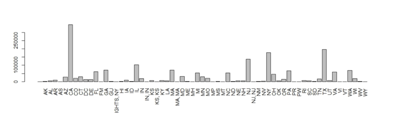
You see the state H1B visa tally from 2012 to 2016.
Next, let’s try to understand the correlation between H1B visas and an outside fact. For simplicity sake, R has a built-in dataset called state.x77. This is a matrix with 50 rows, 1 per state, and facts such as population and life expectancy in the 1977 US Census.
Tip: use a more recent data source in your own analysis.
For now, using the state.x77 is a good example to learn. Examine this built in data set using head().
head(state.x77)Let’s merge this information with the state.tally data into a larger data frame to understand relationships. To do so, create a state.data data frame containing state abbreviations, state.abb, and the old 1977 Census data. Then call on merge passing in the state.tally, and state.data.
You can explicitly declare the state column as the vector to join. Examine a portion of the data frame in the third line by indexing the 15th to 20th rows.
state.data<-data.frame(state=state.abb,state.x77)
state.data<-merge(state.tally,
                  state.data,
                  by='state')
state.data[15:20,]
A basic EDA function is cor: this will print the correlation between two variables.
Remember that correlation ranges from -1 to 1: 0 means the variables have no correlation and are likely unrelated. A number approaching 1 means the values are positively correlated (hopefully) like R programming and income. A negative number means the relationship moves in opposite directions, such as R programming and having a social life!
This code applies cor to the 1977 state population and the current H1B tallies. Remember, the code is meant to illustrate how to perform the analysis despite the temporal mismatch. You can change $Population to reference another vector in the data frame.
cor(state.data$Population, state.data$h1b)Another way to investigate variable relationships is with a scatterplot, particularly a scatterplot matrix. Use pairs() to plot a scatterplot matrix quickly. The code below uses a formula to define the relationships. Each column is declared individually with a plus sign in between. The data parameter accepts the data frame and main simply states the plot title.
pairs(~ h1b + Population + Income,
      data = state.data,
      main='h1b relationships')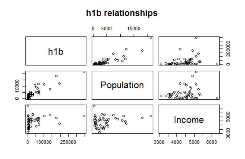
You see that this scatterplot matrix visualizes H1B tallies to state Population and Income.
You can observe a relationship between Population and h1b. This makes intuitive sense as more populated states would have more job opportunities needing an H1B visa.
To “zoom” into a single plot from the matrix simply call plot() and pass in the two variables.
plot(state.data$Income,state.data$h1b,
main = 'Income to H1B')You’ve only begun our H1B visa exploration! This data set is very rich and in the next post you will explore the salary data, get rid of outliers and make more compelling ggplot2 visuals.
You will also build on these EDA concepts by exploring the H1B status over time and also top employers. One of the cool visuals that I will already show you is called a box plot that shows the salary distributions by H1B visa status using this code:
ggplot(h1b.data) +
geom_boxplot(aes(factor(case_status),base_salary,fill=as.factor(case_status))) +
  ylim(0,100000) +
  theme_gdocs() +
  scale_fill_gdocs() +
  theme(axis.text.x=element_blank())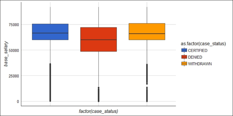
Stay tuned for another part in the "Exploring H-1B Data with R" tutorial series! In the meantime, consider checking out our R data frame tutorial, our Importing Data in R course or our Data Manipulation in R with dplyr course.
R Courses
Course
Course
Course
Tutorial
Arvid Kingl
Tutorial
Filip Schouwenaars
Tutorial
Karlijn Willems
Tutorial
Ted Kwartler
Tutorial
Sicelo Masango
code-along
Ishmael Rico