Cours
Introduction
Importing data is one of the most essential and very first steps in any data related problem. The ability to import the data correctly is a must-have skill for every aspiring data scientist.
Data exists in many different forms, and not only should you know how to import various data formats but also how to analyze and manipulate the data to gain useful insights.
pandas is an open source Python library which is easy-to-use, provides high-performance, and a data analysis tool for various data formats.
It gives you the capability to read various types of data formats like CSV, JSON, Excel, Pickle, etc. It allows you to represent your data in a row and column tabular fashion, which makes the data readable and presentable.
pandas represent the data in a DataFrame form and provide you with extensive usage for data analysis and data manipulation. Once you start making sense out of the data using the various functionalities in pandas, you can then use this data for analyzing, forecasting, classifying, and much more!
pandas has an input and output API which has a set of top-level reader and writer functions. The reader function is accessed with pandas.read_json() that returns a pandas object, and the writer function is accessed with pandas.to_json() which is an object method.
DataFrame has a Reader and a Writer function. The Reader function allows you to read the different data formats, while the Writer function enables you to save the data in a particular format.
Below are data formats that DataFrame supports, which means if your data is in any of the below forms, you can use pandas to load that data format and even write into a particular format.
In today's tutorial, you will be working on a few of the above format types like JSON, HTML, and Pickle.
Note: Check out this tutorial to learn how to read CSV files using pandas.
Loading JSON Data
JSON, also known as JavaScript Object Notation, is a data-interchange text-serialization format. JSON is easy to read and write. It is based on a subset of the JavaScript Programming Language but uses conventions from Python, and many other languages outside of Python.
JSON is mostly used to store unstructured data, and SQL databases have a tough time saving it. JSON makes the data accessible for the machines to read.
JSON is mainly built on two structures:
-
A collection of key/value pairs. In Python, a key/value pair is referred to as a
Dictionary, and akeyis a unique attribute, whereas values are not. -
An ordered list of values. The ordered list can also sometimes be a list of lists. Lists in Python are a set of values which can be a string, integer, etc.
So let's now see how you can load the JSON data in multiple ways.
The first JSON dataset is from this link. The data is in a key-value dictionary format. There are a total of three keys: namely integer, datetime, and category.
- First, you will import the
pandaslibrary and then pass theURLto thepd.read_json()which will return a dataframe. The columns of the dataframes represent the keys, and the rows are the values of the JSON.
import pandas as pd

json = pd.read_json('https://raw.githubusercontent.com/chrisalbon/simulated_datasets/master/data.json')
Let's quickly print the last few rows of the JSON that you read using the .tail() function.
json.tail(6)
| integer | datetime | category | |
|---|---|---|---|
| 94 | 5 | 2015-01-01 00:01:34 | 0 |
| 95 | 9 | 2015-01-01 00:01:35 | 0 |
| 96 | 8 | 2015-01-01 00:01:36 | 0 |
| 97 | 6 | 2015-01-01 00:01:37 | 0 |
| 98 | 8 | 2015-01-01 00:01:38 | 0 |
| 99 | 1 | 2015-01-01 00:01:39 | 0 |
json.shape
(100, 3)
From the above output, you can see that there are three total columns: integer, datetime, and category. Also, there are 100 samples in the dataset as verified from the .shape method which returned a 100 x 3 output.
- Writing a JSON
Writing the JSON data is as simple as reading and is one line of code. Instead of read_json() you will use to_json() with a filename and that's all!
json.to_json('dataframe.json')
- Parsing Nested JSON as a String
Next, you will use another type of JSON dataset, which is not as simple. It is a nested JSON structure. Nested JSON structure means that each key can have more keys associated with it.
Let's see the example dataset to understand it better.
nested_json = """{
   "article": [

      {
         "id":"01",
         "language": "JSON",
         "edition": "first",
         "author": "Allen"
      },

      {
         "id":"02",
         "language": "Python",
         "edition": "second",
         "author": "Aditya Sharma"
      }
   ],

   "blog":[
   {
       "name": "Datacamp",
       "URL":"datacamp.com"
   }
   ]
}"""
In the above dataset, you can observe that article and blog are two primary keys under which there are values of these keys. These values have their own key-value pair combination.
Note that the above dataset is enclosed with double-quotes and is in the form of a string.
Reading a nested JSON can be done in multiple ways.
First, you will use the json.loads function to read a JSON string by passing the data variable as a parameter to it. Then, you will use the json_normalize function to flatten the nested JSON data into a table.
You will import the json_normalize function from the pandas.io.json library.
import json
from pandas.io.json import json_normalize

nested = json.loads(nested_json)
nested
{'article': [{'id': '01',
   'language': 'JSON',
   'edition': 'first',
   'author': 'Allen'},
  {'id': '02',
   'language': 'Python',
   'edition': 'second',
   'author': 'Aditya Sharma'}],
 'blog': [{'name': 'Datacamp', 'URL': 'datacamp.com'}]}
Next, you will flatten the JSON using the normalize function. You will pass in the complete data for now and see how it looks.
nested_full = json_normalize(nested)
nested_full
| article | blog | |
|---|---|---|
| 0 | [{'id': '01', 'language': 'JSON', 'edition': '... | [{'name': 'Datacamp', 'URL': 'datacamp.com'}] |
Great! So as you can see from the above output, the primary keys are the columns of the dataframe while the keys represent the row.
However, the output looks a little clumsy, right? Let's see how you can further divide it into multiple dataframes.
You will again pass in the json.loads output to json_normalize but this time you will specify an extra element called record_path.
blog = json_normalize(nested,record_path ='blog')
blog
| URL | name | |
|---|---|---|
| 0 | datacamp.com | Datacamp |
article = json_normalize(nested,record_path ='article')
article
| author | edition | id | language | |
|---|---|---|---|---|
| 0 | Allen | first | 01 | JSON |
| 1 | Aditya Sharma | second | 02 | Python |
From the above outputs, you can observe that the primary keys are now divided into two different dataframes where the column names have now become the keys that were nested inside the primary keys as a key-value pair. Amazing, right?
Lastly, to wrap up JSON data loading, let's quickly find out how you can read JSON as a file and not as a string.
- Reading a JSON as a File
nested_json = {
   "article": [

      {
         "id":"01",
         "language": "JSON",
         "edition": "first",
         "author": "Allen"
      },

      {
         "id":"02",
         "language": "Python",
         "edition": "second",
         "author": "Aditya Sharma"
      }
   ],

   "blog":[
   {
       "name": "Datacamp",
       "URL":"datacamp.com"
   }
   ]
}
If you notice in the above cell, there are no double-quotes in the start and end of the data, which means you will be treating this data as a file and read it.
You can achieve this with just one line of code. Let's find out how!
json_file = pd.DataFrame.from_dict(json_normalize(nested_json))
json_file
| article | blog | |
|---|---|---|
| 0 | [{'id': '01', 'language': 'JSON', 'edition': '... | [{'name': 'Datacamp', 'URL': 'datacamp.com'}] |
From the above output, you can see that the output is similar to when you read JSON as a string. The only change here is that you use pandas to both parse and flatten the JSON. Since the JSON is a dictionary you use the .from_dict() function.
Loading HTML Data
HTML is a Hypertext Markup Language that is mainly used for created web applications and pages. It tries to describe the structure of the web page semantically. The web browser receives an HTML document from a web server and renders it to a multimedia web page.
For web applications, HTML is used with cascading style sheets (CSS) while at the server end it collaborates with various web server frameworks like Flask, Django, etc.
HTML uses tags to define each block of code like a <p></p> tag for the start and end of a paragraph, <image></image> tag for adding content to the web page as an image and similarly there are many tags that together collate to form an HTML web page.
To read an HTML file, pandas dataframe looks for a tag. That tag is called a <td></td> tag. This tag is used for defining a table in HTML.
pandas uses read_html() to read the HTML document.
So, whenever you pass an HTML to pandas and expect it to output a nice looking dataframe, make sure the HTML page has a table in it!
- About the Data: You will be using a
Cryptocurrencywebsite as an HTML dataset that has various crypto coins on it and has various details about each coin like:- Last price of the coin (
Last price) - Whether the coin price has increased or decreased (in percentage
%) - The volume of 24 hours (how many coins were traded
24 volume) - Total number of coins (
# Coins)
- Last price of the coin (
So, let's get started!
You will first import requests library which will help you in sending a request to the URL from where you want to fetch the HTML content.
import requests
url = 'https://www.worldcoinindex.com/'
crypto_url = requests.get(url)
crypto_url
<Response [200]>
So, until now, you defined the URL and then using requests.get() you sent a request to that URL and received a response as an acknowledgement [200] OK which means that you were able to connect with that web server.
Now, to read the content of the HTML web page, all you need to do is call crypto_url.text which will give you the HTML code of that cryptocurrency web page.
Feel free to run the command crypto_url.text to see the output.
Finally, you will pass crypto_url.text to the pd.read_html() function which will return you a list of dataframes where each element in that list is a table (dataframe) the cryptocurrency webpage has in it.
crypto_data = pd.read_html(crypto_url.text)
Let's print the length and the type of the dataframe. The type should be a list.
len(crypto_data), type(crypto_data)
(1, list)
From the above output, it is clear that there is only 1 table with a type list.
crypto_data = crypto_data[0]
Let's remove the first and second column since they do not have any useful information in them and keep all the rows.
crypto_final = crypto_data.iloc[:,2:]
Finally, it's time to print the cryptocurrency dataframe!
crypto_final.head()
| Name | Ticker | Last price | % | 24 high | 24 low | Price Charts 7d | 24 volume | # Coins | Market cap | |
|---|---|---|---|---|---|---|---|---|---|---|
| 0 | bitcoin | BTC | $ 8,008.027 | +1.83% | $ 8,056.630 | $ 7,812.784 | NaN | $ 12.04B | 17.71M | $ 141.89B |
| 1 | ethereum | ETH | $ 251.72335 | +2.68% | $ 253.84721 | $ 242.95687 | NaN | $ 6.93B | 106.20M | $ 26.73B |
| 2 | litecoin | LTC | $ 98.633851 | +11.08% | $ 99.946324 | $ 88.618815 | NaN | $ 3.46B | 61.91M | $ 6.10B |
| 3 | bitcoincash | BCH | $ 411.94075 | +2.31% | $ 418.60850 | $ 394.18927 | NaN | $ 2.10B | 17.79M | $ 7.33B |
| 4 | eos | EOS | $ 6.4230717 | +6.05% | $ 6.4765695 | $ 6.0264079 | NaN | $ 2.06B | 1.01B | $ 6.50B |
From the above table, you can observe that Bitcoin has the most Market Cap.
Dropping NaN (Not a Number)
There are some values in the dataframe that are not real values, so let's quickly remove them from the table.
However, first, let's completely drop (delete) the Price Charts 7d column since it is entirely NaN and has zero information in it.
del crypto_final['Price Charts 7d']
crypto_final.head()
| Name | Ticker | Last price | % | 24 high | 24 low | 24 volume | # Coins | Market cap | |
|---|---|---|---|---|---|---|---|---|---|
| 0 | bitcoin | BTC | $ 8,008.027 | +1.83% | $ 8,056.630 | $ 7,812.784 | $ 12.04B | 17.71M | $ 141.89B |
| 1 | ethereum | ETH | $ 251.72335 | +2.68% | $ 253.84721 | $ 242.95687 | $ 6.93B | 106.20M | $ 26.73B |
| 2 | litecoin | LTC | $ 98.633851 | +11.08% | $ 99.946324 | $ 88.618815 | $ 3.46B | 61.91M | $ 6.10B |
| 3 | bitcoincash | BCH | $ 411.94075 | +2.31% | $ 418.60850 | $ 394.18927 | $ 2.10B | 17.79M | $ 7.33B |
| 4 | eos | EOS | $ 6.4230717 | +6.05% | $ 6.4765695 | $ 6.0264079 | $ 2.06B | 1.01B | $ 6.50B |
Now let's remove the NaN's.
crypto_final = crypto_final.dropna()
Visualizing the Crypto Coins (Ticker) Vs. Percentage Increase/Decrease in Price (%)
Let's first import matplotlib for plotting the graph.
import matplotlib.pyplot as plt
%matplotlib inline
The % column has a type string, and you need to convert the type string to float. First, you will remove the % sign from the column and then convert the type of the % column to float.
crypto_final['%'] = crypto_final['%'].apply(lambda x: x.strip('%'))
crypto_final['%'] = crypto_final['%'].astype('float')
Let's now plot the data.
plt.figure()
plt.figure(figsize=(16,10))
x = crypto_final.iloc[:20]['Ticker']
y = crypto_final.iloc[:20]['%']
plt.xticks(fontsize=12)
plt.yticks(fontsize=14)
plt.xlabel('Percentage Increase/Decrease in Price',fontsize=20)
plt.ylabel('Ticker',fontsize=20)

plt.plot(x,y,label='% Increase/Decrease in Price')
plt.legend(loc='lower left',prop={'size': 15})
<matplotlib.legend.Legend at 0x1298a9630>

<Figure size 432x288 with 0 Axes>
From the above graph, you can observe that the Litecoin (LTC) and Huobitoken (HT) have the maximum increase in the price and on the other hand, Maticnetwork (MATIC) and Waves have the maximum decrease in the price of the crypto coins.
Loading Pickle Data
Pickle is a Python-specific binary serialization format which is not human-readable, unlike JSON. It is used for serializing and deserializing an object structure of Python. It serializes the object and Pickles it to save it on a disk. It converts the object like DataFrame, list, dictionary, etc. into a character stream.
The best part about Pickle is that it can store various kinds of Python data types.
Pickle is widely used for storing trained machine learning algorithm instances. Like JSON, Pickle also has handy functions like pickle.load() for loading a Pickle format file, and pickle.dump() for saving a Pickle or any other format in Pickle format.
Another import advantage of using Pickle is that Saving the dataframe as a Pickle file required less space on the disk and keeps the type of the data intact when reloaded.
So, let's quickly pickle the cryptocurrency dataframe you constructed earlier, and then you will read that pickled object using pandas.
import pickle
You will use pickle.dump to save the dataframe as a Pickle object and use the protocol as HIGHEST_PROTOCOL, which is backward compatible with Python 2 as well.
with open('crypto_final.pickle', 'wb') as sub_data:
    pickle.dump(crypto_final, sub_data, protocol=pickle.HIGHEST_PROTOCOL)
Finally, you will use the pandas read_pickle function to convert the pickle object into a dataframe.
crypto_final = pd.read_pickle('crypto_final.pickle')
crypto_final.head()
| Name | Ticker | Last price | % | 24 high | 24 low | 24 volume | # Coins | Market cap | |
|---|---|---|---|---|---|---|---|---|---|
| 0 | bitcoin | BTC | $ 7,776.567 | +1.81% | $ 7,870.205 | $ 7,506.518 | $ 12.70B | 17.71M | $ 137.78B |
| 1 | ethereum | ETH | $ 241.81372 | -0.97% | $ 245.57293 | $ 232.62523 | $ 7.47B | 106.18M | $ 25.67B |
| 2 | litecoin | LTC | $ 88.062811 | +0.33% | $ 88.946501 | $ 85.248641 | $ 2.59B | 61.90M | $ 5.45B |
| 3 | bitcoincash | BCH | $ 388.76089 | +0.06% | $ 398.27697 | $ 370.29831 | $ 2.33B | 17.79M | $ 6.91B |
| 4 | eos | EOS | $ 5.9327948 | -0.41% | $ 6.0163442 | $ 5.7789154 | $ 1.99B | 1.01B | $ 6.00B |
Wow! Isn't that amazing? How straightforward that was. Moreover, with Pickle, you do not have to worry about the datatype conversion errors as the pickle serialization can handle that for you!
Go Further
Congratulations on finishing the tutorial.
This tutorial was a good starting point on how you can load different data formats in Python with the help of pandas.
There are still many data formats like Excel, SQL, HDF5, etc., that fall under the pandas data import umbrella. You should get your hands dirty with them by finding some interesting public datasets in these data formats and try experimenting with them.
If you would like to learn more about DataFrames in pandas, take DataCamp's data manipulation with pandas interactive course. DataCamp also has several other handy pandas tutorials covering joining dataframes, implementing moving averages and using the apply method. Or, if you're completely new to pandas, start with this beginners guide to pandas tutorial.
References:
Please feel free to ask any questions related to this tutorial in the comments section below.


