Course
Intermediate Python
4 hr
1.4M
A moving average, also called a rolling or running average, is used to analyze the time-series data by calculating averages of different subsets of the complete dataset. Since it involves taking the average of the dataset over time, it is also called a moving mean (MM) or rolling mean.
There are various ways in which the rolling average can be calculated, but one such way is to take a fixed subset from a complete series of numbers. The first moving average is calculated by averaging the first fixed subset of numbers, and then the subset is changed by moving forward to the next fixed subset (including the future value in the subgroup while excluding the previous number from the series).
The moving average is mostly used with time series data to capture the short-term fluctuations while focusing on longer trends.
A few examples of time series data can be stock prices, weather reports, air quality, gross domestic product, employment, etc.
In general, the moving average smoothens the data.
Moving average is a backbone to many algorithms, and one such algorithm is Autoregressive Integrated Moving Average Model (ARIMA), which uses moving averages to make time series data predictions.
There are various types of moving averages:
Simple Moving Average (SMA): Simple Moving Average (SMA) uses a sliding window to take the average over a set number of time periods. It is an equally weighted mean of the previous n data.
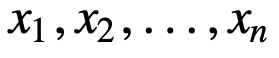
To understand SMA further, lets take an example, a sequence of n values:
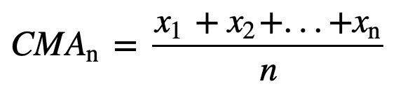
then the equally weighted rolling average for n data points will be essentially the mean of the previous M data-points, where M is the size of the sliding window:
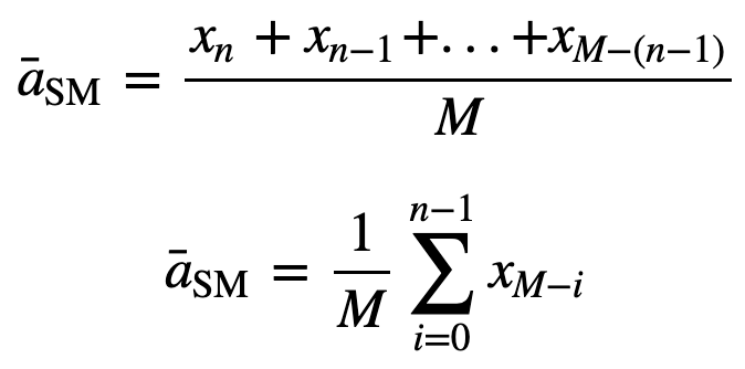
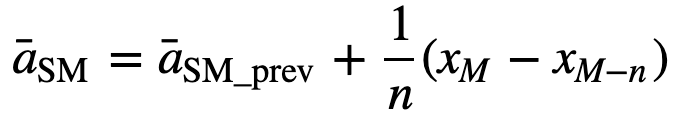
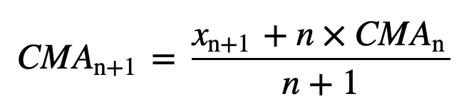
Similarly, for calculating succeeding rolling average values, a new value will be added into the sum, and the previous time period value will be dropped out, since you have the average of previous time periods so full summation each time is not required:
Since EMAs give a higher weight on recent data than on older data, they are more responsive to the latest price changes as compared to SMAs, which makes the results from EMAs more timely and hence EMA is more preferred over other techniques.
Enough of theory, right? Let's jump to the practical implementation of the moving average.
First, let's create dummy time series data and try implementing SMA using just Python.
Assume that there is a demand for a product and it is observed for 12 months (1 Year), and you need to find moving averages for 3 and 4 months window periods.
Import module
import pandas as pd
import numpy as np
product = {'month' : [1,2,3,4,5,6,7,8,9,10,11,12],'demand':[290,260,288,300,310,303,329,340,316,330,308,310]}
df = pd.DataFrame(product)df.head()Run and edit the code from this tutorial online
Run code| month | demand | |
|---|---|---|
| 0 | 1 | 290 |
| 1 | 2 | 260 |
| 2 | 3 | 288 |
| 3 | 4 | 300 |
| 4 | 5 | 310 |
Let's calculate SMA for a window size of 3, which means you will consider three values each time to calculate the moving average, and for every new value, the oldest value will be ignored.
To implement this, you will use pandas iloc function, since the demand column is what you need, you will fix the position of that in the iloc function while the row will be a variable i which you will keep iterating until you reach the end of the dataframe.
for i in range(0,df.shape[0]-2):
df.loc[df.index[i+2],'SMA_3'] = np.round(((df.iloc[i,1]+ df.iloc[i+1,1] +df.iloc[i+2,1])/3),1)| month | demand | SMA_3 | |
|---|---|---|---|
| 0 | 1 | 290 | NaN |
| 1 | 2 | 260 | NaN |
| 2 | 3 | 288 | 279.3 |
| 3 | 4 | 300 | 282.7 |
| 4 | 5 | 310 | 299.3 |
For a sanity check, let's also use the pandas in-built rolling function and see if it matches with our custom python based simple moving average.
df['pandas_SMA_3'] = df.iloc[:,1].rolling(window=3).mean()df.head()| month | demand | SMA_3 | pandas_SMA_3 | |
|---|---|---|---|---|
| 0 | 1 | 290 | NaN | NaN |
| 1 | 2 | 260 | NaN | NaN |
| 2 | 3 | 288 | 279.3 | 279.333333 |
| 3 | 4 | 300 | 282.7 | 282.666667 |
| 4 | 5 | 310 | 299.3 | 299.333333 |
Cool, so as you can see, the custom and pandas moving averages match exactly, which means your implementation of SMA was correct.
Let's also quickly calculate the simple moving average for a window_size of 4.
for i in range(0,df.shape[0]-3):
    df.loc[df.index[i+3],'SMA_4'] = np.round(((df.iloc[i,1]+ df.iloc[i+1,1] +df.iloc[i+2,1]+df.iloc[i+3,1])/4),1)
df.head()
| month | demand | SMA_3 | pandas_SMA_3 | SMA_4 | |
|---|---|---|---|---|---|
| 0 | 1 | 290 | NaN | NaN | NaN |
| 1 | 2 | 260 | NaN | NaN | NaN |
| 2 | 3 | 288 | 279.3 | 279.333333 | NaN |
| 3 | 4 | 300 | 282.7 | 282.666667 | 284.5 |
| 4 | 5 | 310 | 299.3 | 299.333333 | 289.5 |
df['pandas_SMA_4'] = df.iloc[:,1].rolling(window=4).mean()
df.head()
| month | demand | SMA_3 | pandas_SMA_3 | SMA_4 | pandas_SMA_4 | |
|---|---|---|---|---|---|---|
| 0 | 1 | 290 | NaN | NaN | NaN | NaN |
| 1 | 2 | 260 | NaN | NaN | NaN | NaN |
| 2 | 3 | 288 | 279.3 | 279.333333 | NaN | NaN |
| 3 | 4 | 300 | 282.7 | 282.666667 | 284.5 | 284.5 |
| 4 | 5 | 310 | 299.3 | 299.333333 | 289.5 | 289.5 |
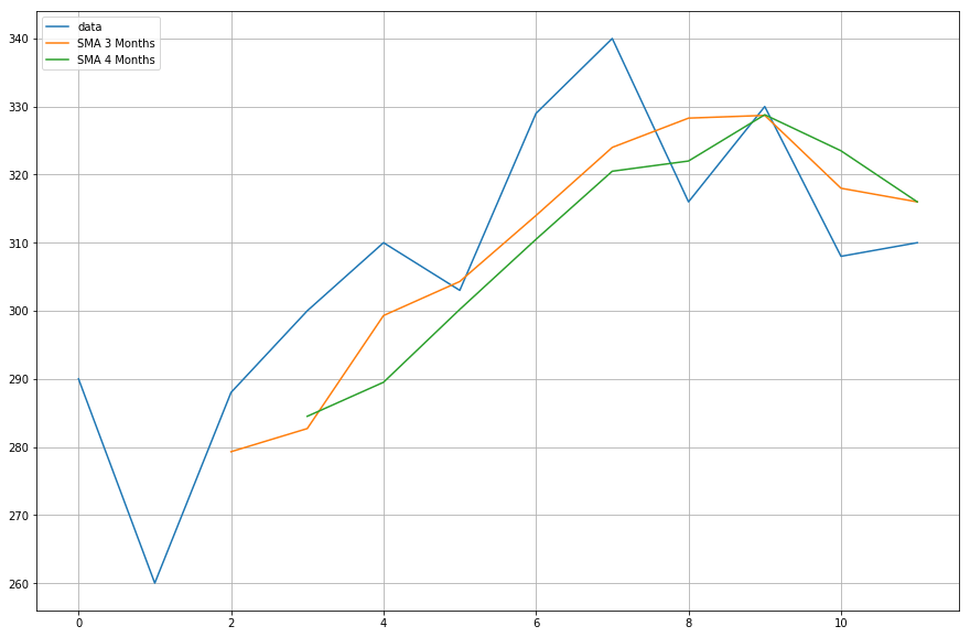
Now, you will plot the data of the moving averages that you calculated.
import matplotlib.pyplot as plt
%matplotlib inline
plt.figure(figsize=[15,10])
plt.grid(True)
plt.plot(df['demand'],label='data')
plt.plot(df['SMA_3'],label='SMA 3 Months')
plt.plot(df['SMA_4'],label='SMA 4 Months')
plt.legend(loc=2)
<matplotlib.legend.Legend at 0x11fe15080>
I think we are now ready to move to a real dataset.
For cumulative moving average, let's use an air quality dataset which can be downloaded from this link.
df = pd.read_csv("AirQualityUCI/AirQualityUCI.csv", sep = ";", decimal = ",")
df = df.iloc[ : , 0:14]
df.head()
| Date | Time | CO(GT) | PT08.S1(CO) | NMHC(GT) | C6H6(GT) | PT08.S2(NMHC) | NOx(GT) | PT08.S3(NOx) | NO2(GT) | PT08.S4(NO2) | PT08.S5(O3) | T | RH | |
|---|---|---|---|---|---|---|---|---|---|---|---|---|---|---|
| 0 | 10/03/2004 | 18.00.00 | 2.6 | 1360.0 | 150.0 | 11.9 | 1046.0 | 166.0 | 1056.0 | 113.0 | 1692.0 | 1268.0 | 13.6 | 48.9 |
| 1 | 10/03/2004 | 19.00.00 | 2.0 | 1292.0 | 112.0 | 9.4 | 955.0 | 103.0 | 1174.0 | 92.0 | 1559.0 | 972.0 | 13.3 | 47.7 |
| 2 | 10/03/2004 | 20.00.00 | 2.2 | 1402.0 | 88.0 | 9.0 | 939.0 | 131.0 | 1140.0 | 114.0 | 1555.0 | 1074.0 | 11.9 | 54.0 |
| 3 | 10/03/2004 | 21.00.00 | 2.2 | 1376.0 | 80.0 | 9.2 | 948.0 | 172.0 | 1092.0 | 122.0 | 1584.0 | 1203.0 | 11.0 | 60.0 |
| 4 | 10/03/2004 | 22.00.00 | 1.6 | 1272.0 | 51.0 | 6.5 | 836.0 | 131.0 | 1205.0 | 116.0 | 1490.0 | 1110.0 | 11.2 | 59.6 |
Preprocessing is an essential step whenever you are working with data. For numerical data one of the most common preprocessing steps is to check for NaN (Null) values. If there are any NaN values, you can replace them with either 0 or average or preceding or succeeding values or even drop them. Though replacing is normally a better choice over dropping them, since this dataset has few NULL values, dropping them will not affect the continuity of the series.
df.isna().sum()
Date             114
Time             114
CO(GT)           114
PT08.S1(CO)      114
NMHC(GT)         114
C6H6(GT)         114
PT08.S2(NMHC)    114
NOx(GT)          114
PT08.S3(NOx)     114
NO2(GT)          114
PT08.S4(NO2)     114
PT08.S5(O3)      114
T                114
RH               114
dtype: int64
From the above output, you can observe that there are around 114 NaN values across all columns, however you will figure out that they are all at the end of the time-series, so let's quickly drop them.
df.dropna(inplace=True)
df.isna().sum()
Date             0
Time             0
CO(GT)           0
PT08.S1(CO)      0
NMHC(GT)         0
C6H6(GT)         0
PT08.S2(NMHC)    0
NOx(GT)          0
PT08.S3(NOx)     0
NO2(GT)          0
PT08.S4(NO2)     0
PT08.S5(O3)      0
T                0
RH               0
dtype: int64
You will be applying cumulative moving average on the Temperature column (T), so let's quickly separate that column out from the complete data.
df_T = pd.DataFrame(df.iloc[:,-2])
df_T.head()
| T | |
|---|---|
| 0 | 13.6 |
| 1 | 13.3 |
| 2 | 11.9 |
| 3 | 11.0 |
| 4 | 11.2 |
Now, you will use the pandas expanding method fo find the cumulative average of the above data. If you recall from the introduction, unlike the simple moving average, the cumulative moving average considers all of the preceding values when calculating the average.
df_T['CMA_4'] = df_T.expanding(min_periods=4).mean()
df_T.head(10)
| T | CMA_4 | |
|---|---|---|
| 0 | 13.6 | NaN |
| 1 | 13.3 | NaN |
| 2 | 11.9 | NaN |
| 3 | 11.0 | 12.450000 |
| 4 | 11.2 | 12.200000 |
| 5 | 11.2 | 12.033333 |
| 6 | 11.3 | 11.928571 |
| 7 | 10.7 | 11.775000 |
| 8 | 10.7 | 11.655556 |
| 9 | 10.3 | 11.520000 |
Time series data is plotted with respect to the time, so let's combine the date and time column and convert it into a datetime object. To achieve this, you will use the datetime module from python (Source: Time Series Tutorial).
import datetime

df['DateTime'] = (df.Date) + ' ' + (df.Time)
df.DateTime = df.DateTime.apply(lambda x: datetime.datetime.strptime(x, '%d/%m/%Y %H.%M.%S'))
Let's change the index of the temperature dataframe with datetime.
df_T.index = df.DateTime
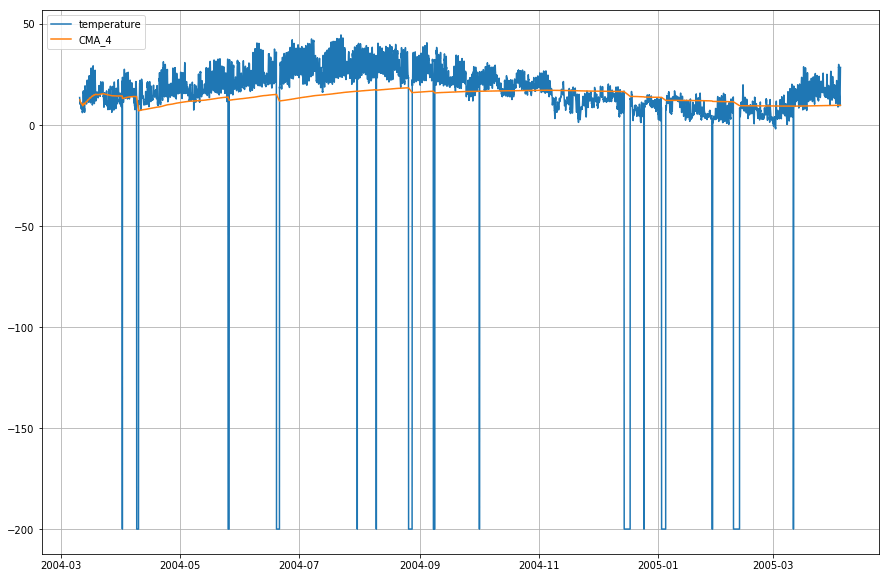
Let's now plot the actual temperature and the cumulative moving average wrt. time.
plt.figure(figsize=[15,10])
plt.grid(True)
plt.plot(df_T['T'],label='temperature')
plt.plot(df_T['CMA_4'],label='CMA_4')
plt.legend(loc=2)
<matplotlib.legend.Legend at 0x1210a2d30>
df_T['EMA'] = df_T.iloc[:,0].ewm(span=40,adjust=False).mean()
df_T.head()
| T | CMA_4 | EMA | |
|---|---|---|---|
| DateTime | |||
| 2004-03-10 18:00:00 | 13.6 | NaN | 13.600000 |
| 2004-03-10 19:00:00 | 13.3 | NaN | 13.585366 |
| 2004-03-10 20:00:00 | 11.9 | NaN | 13.503153 |
| 2004-03-10 21:00:00 | 11.0 | 12.45 | 13.381048 |
| 2004-03-10 22:00:00 | 11.2 | 12.20 | 13.274655 |
plt.figure(figsize=[15,10])
plt.grid(True)
plt.plot(df_T['T'],label='temperature')
plt.plot(df_T['CMA_4'],label='CMA_4')
plt.plot(df_T['EMA'],label='EMA')
plt.legend(loc=2)
<matplotlib.legend.Legend at 0x14b2a41d0>
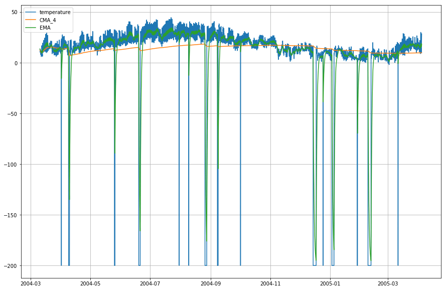
Wow! So as you can observe from the graph above, that the Exponential Moving Average (EMA) does a superb job in capturing the pattern of the data while the Cumulative Moving Average (CMA) lacks by a considerable margin.
Congratulations on finishing the tutorial.
This tutorial was a good starting point on how you can calculate the moving averages of your data and make sense of it.
Try writing the cumulative and exponential moving average python code without using the pandas library. That will give you much more in-depth knowledge about how they are calculated and in what ways are they different from each other.
There is still a lot to experiment. Try calculating the partial auto-correlation between the input data and the moving average, and try to find some relation between the two.
If you would like to learn more about DataFrames in pandas, take DataCamp's pandas Foundations interactive course.
References:
Please feel free to ask any questions related to this tutorial in the comments section below.
Related courses
Course
Course
Course
cheat-sheet
Karlijn Willems
Tutorial
Karlijn Willems
Tutorial
Karlijn Willems
Tutorial
Jason Graham
Tutorial
Aditya Sharma