Python pandas tutorial: The ultimate guide for beginners

Install pandas

Installing pandas is straightforward; just use the pip install command in your terminal. 

pip install pandas

Importing data in pandas

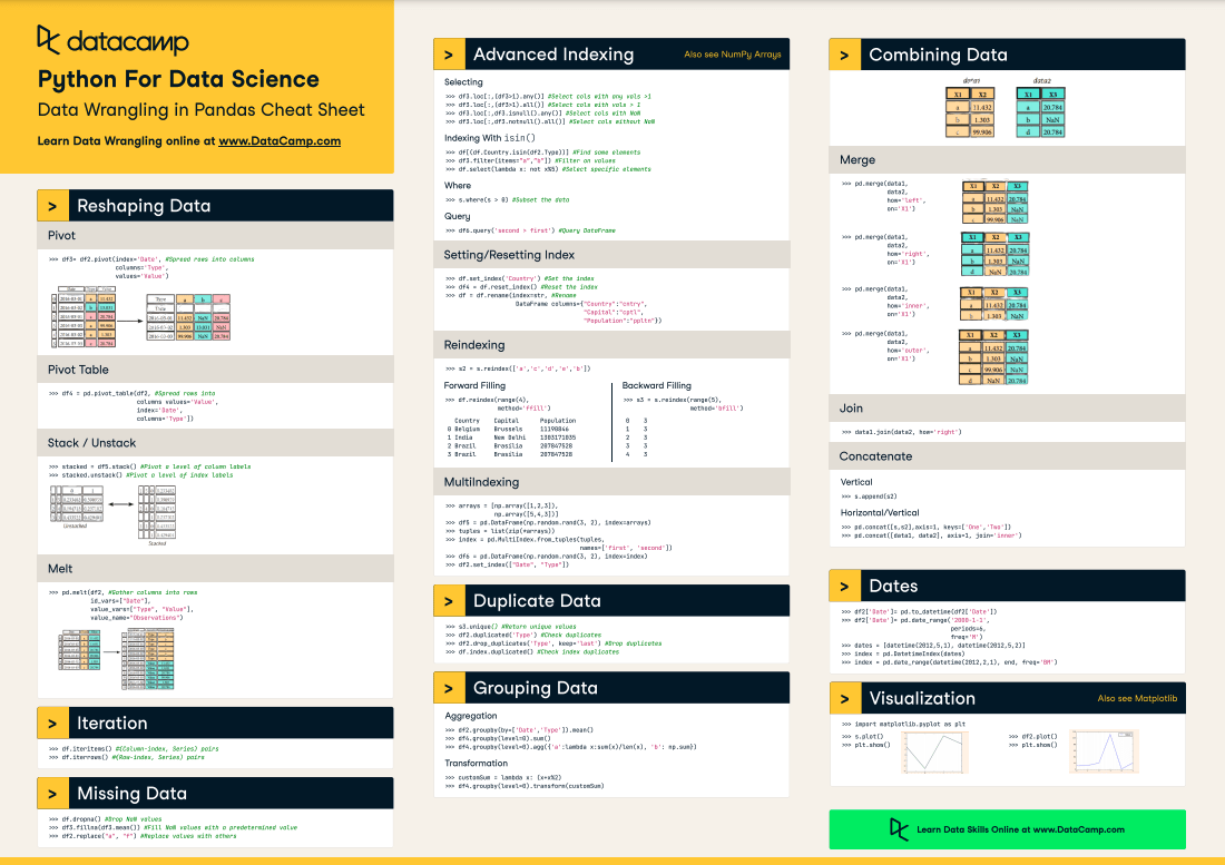
To begin working with pandas, import the pandas Python package as shown below. When importing pandas, the most common alias for pandas is pd.

import pandas as pd

Importing CSV files

Use read_csv() with the path to the CSV file to read a comma-separated values file (see our tutorial on importing data with read_csv() for more detail).

df = pd.read_csv("diabetes.csv")

This read operation loads the CSV file diabetes.csv to generate a pandas Dataframe object df. Throughout this tutorial, you'll see how to manipulate such DataFrame objects. 

Importing text files

Reading text files is similar to CSV files. The only nuance is that you need to specify a separator with the sep argument, as shown below. The separator argument refers to the symbol used to separate rows in a DataFrame. Comma (sep = ","), whitespace(sep = "\s"), tab (sep = "\t"), and colon(sep = ":") are the commonly used separators. Here \s represents a single white space character.

df = pd.read_csv("diabetes.txt", sep="\s")

Importing Excel files (single sheet)

Reading excel files (both XLS and XLSX) is as easy as the read_excel() function, using the file path as an input.

df = pd.read_excel('diabetes.xlsx')

You can also specify other arguments, such as header for to specify which row becomes the DataFrame's header. It has a default value of 0, which denotes the first row as headers or column names. You can also specify column names as a list in the names argument. The index_col (default is None) argument can be used if the file contains a row index.

Note: In a pandas DataFrame or Series, the index is an identifier that points to the location of a row or column in a pandas DataFrame. In a nutshell, the index labels the row or column of a DataFrame and lets you access a specific row or column by using its index (you will see this later on). A DataFrame’s row index can be a range (e.g., 0 to 303), a time series (dates or timestamps), a unique identifier (e.g., employee_ID in an employees table), or other types of data. For columns, it's usually a string (denoting the column name).

Importing Excel files (multiple sheets)

Reading Excel files with multiple sheets is not that different. You just need to specify one additional argument, sheet_name, where you can either pass a string for the sheet name or an integer for the sheet position (note that Python uses 0-indexing, where the first sheet can be accessed with sheet_name = 0)

# Extracting the second sheet since Python uses 0-indexing
df = pd.read_excel('diabetes_multi.xlsx', sheet_name=1)

Importing JSON file

Similar to the read_csv() function, you can use read_json() for JSON file types with the JSON file name as the argument (for more detail read this tutorial on importing JSON and HTML data into pandas). The below code reads a JSON file from disk and creates a DataFrame object df.

df = pd.read_json("diabetes.json")

If you want to learn more about importing data with pandas, check out this cheat sheet on importing various file types with Python. 

Outputting data in pandas

Just as pandas can import data from various file types, it also allows you to export data into various formats. This happens especially when data is transformed using pandas and needs to be saved locally on your machine. Below is how to output pandas DataFrames into various formats.

Outputting a DataFrame into a CSV file

A pandas DataFrame (here we are using df) is saved as a CSV file using the .to_csv() method. The arguments include the filename with path and index – where index = True implies writing the DataFrame’s index.

df.to_csv("diabetes_out.csv", index=False)

Outputting a DataFrame into a JSON file

Export DataFrame object into a JSON file by calling the .to_json() method.

df.to_json("diabetes_out.json")

Note: A JSON file stores a tabular object like a DataFrame as a key-value pair. Thus you would observe repeating column headers in a JSON file.

Outputting a DataFrame into a text file

As with writing DataFrames to CSV files, you can call .to_csv(). The only differences are that the output file format is in .txt, and you need to specify a separator using the sep argument.

df.to_csv('diabetes_out.txt', header=df.columns, index=None, sep=' ')

Outputting a DataFrame into an Excel file

Call .to_excel() from the DataFrame object to save it as a “.xls” or “.xlsx” file.

df.to_excel("diabetes_out.xlsx", index=False)

Viewing and understanding DataFrames using pandas 

After reading tabular data as a DataFrame, you would need to have a glimpse of the data. You can either view a small sample of the dataset or a summary of the data in the form of summary statistics.

How to view data using .head() and .tail()

You can view the first few or last few rows of a DataFrame using the .head() or .tail() methods, respectively. You can specify the number of rows through the n argument (the default value is 5).

df.head()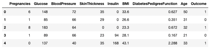

First five rows of the DataFrame 

df.tail(n = 10)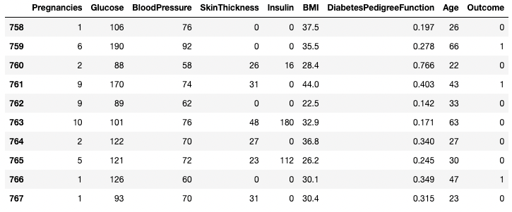

First 10 rows of the DataFrame 

Understanding data using .describe()

The .describe() method prints the summary statistics of all numeric columns, such as count, mean, standard deviation, range, and quartiles of numeric columns.

df.describe()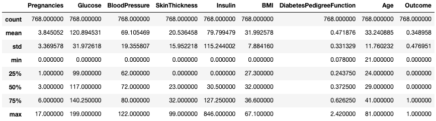

Get summary statistics with .describe()

It gives a quick look at the scale, skew, and range of numeric data.

You can also modify the quartiles using the percentiles argument. Here, for example, we’re looking at the 30%, 50%, and 70% percentiles of the numeric columns in DataFrame df.

df.describe(percentiles=[0.3, 0.5, 0.7])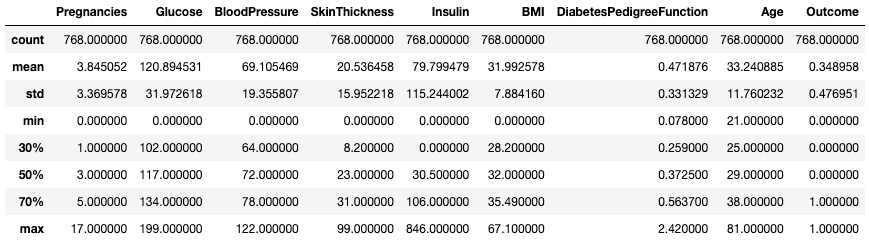

Get summary statistics with specific percentiles 

You can also isolate specific data types in your summary output by using the include argument. Here, for example, we’re only summarizing the columns with the integer data type. 

df.describe(include=[int])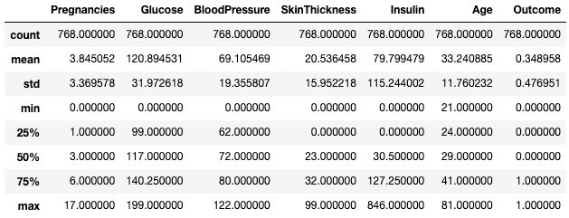

Get summary statistics of integer columns only 

Similarly, you might want to exclude certain data types using exclude argument.

df.describe(exclude=[int])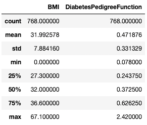

Get summary statistics of non-integer columns only 

Often, practitioners find it easy to view such statistics by transposing them with the .T attribute.

df.describe().T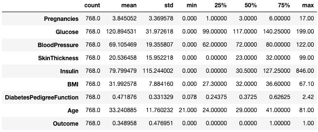

Transpose summary statistics with .T

For more on describing DataFrames, check out the following cheat sheet.

Understanding data using .info()

The .info() method is a quick way to look at the data types, missing values, and data size of a DataFrame. Here, we’re setting the show_counts argument to True, which gives a few over the total non-missing values in each column. We’re also setting memory_usage to True, which shows the total memory usage of the DataFrame elements. When verbose is set to True, it prints the full summary from .info(). 

df.info(show_counts=True, memory_usage=True, verbose=True)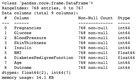

Understanding your data using .shape

The number of rows and columns of a DataFrame can be identified using the .shape attribute of the DataFrame. It returns a tuple (row, column) and can be indexed to get only rows, and only columns count as output.

df.shape # Get the number of rows and columns
df.shape[0] # Get the number of rows only
df.shape[1] # Get the number of columns only

(768,9)
768
9

Get all columns and column names

Calling the .columns attribute of a DataFrame object returns the column names in the form of an Index object. As a reminder, a pandas index is the address/label of the row or column.

df.columns

It can be converted to a list using a list() function.

list(df.columns)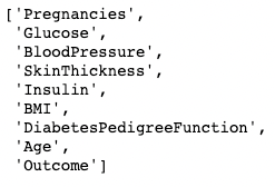

Checking for missing values in pandas with .isnull()

The sample DataFrame does not have any missing values. Let's introduce a few to make things interesting. The .copy() method makes a copy of the original DataFrame. This is done to ensure that any changes to the copy don’t reflect in the original DataFrame. Using .loc (to be discussed later), you can set rows two to five of the Pregnancies column to NaN values, which denote missing values.

df2 = df.copy()
df2.loc[2:5,'Pregnancies'] = None
df2.head(7)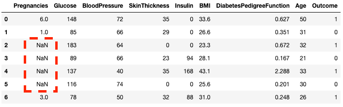

You can see, that now rows 2 to 5 are NaN

You can check whether each element in a DataFrame is missing using the .isnull() method.

df2.isnull().head(7)

Given it's often more useful to know how much missing data you have, you can combine .isnull() with .sum() to count the number of nulls in each column.

df2.isnull().sum()

Pregnancies                 4
Glucose                     0
BloodPressure               0
SkinThickness               0
Insulin                     0
BMI                         0
DiabetesPedigreeFunction    0
Age                         0
Outcome                     0
dtype: int64

You can also do a double sum to get the total number of nulls in the DataFrame.

df2.isnull().sum().sum()

4

Slicing and Extracting Data in pandas

The pandas package offers several ways to subset, filter, and isolate data in your DataFrames. Here, we'll see the most common ways.

Isolating one column using [ ] 

You can isolate a single column using a square bracket [ ] with a column name in it. The output is a pandas Series object. A pandas Series is a one-dimensional array containing data of any type, including integer, float, string, boolean, python objects, etc. A DataFrame is comprised of many series that act as columns.

df['Outcome']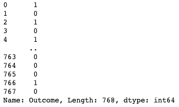

Isolating one column in pandas

Isolating two or more columns using [[ ]] 

You can also provide a list of column names inside the square brackets to fetch more than one column. Here, square brackets are used in two different ways. We use the outer square brackets to indicate a subset of a DataFrame, and the inner square brackets to create a list.

df[['Pregnancies', 'Outcome']]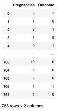

Isolating two columns in pandas

Isolating one row using [ ] 

A single row can be fetched by passing in a boolean series with one True value. In the example below, the second row with index = 1 is returned. Here, .index returns the row labels of the DataFrame, and the comparison turns that into a Boolean one-dimensional array.

df[df.index==1]

Isolating one row in pandas

Isolating two or more rows using [ ] 

Similarly, two or more rows can be returned using the .isin() method instead of a == operator.

df[df.index.isin(range(2,10))]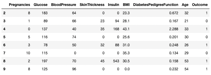

Isolating specific rows in pandas

Using .loc[] and .iloc[] to fetch rows

You can fetch specific rows by labels or conditions using .loc[] and .iloc[] ("location" and "integer location"). .loc[] uses a label to point to a row, column or cell, whereas .iloc[] uses the numeric position. To understand the difference between the two, let’s modify the index of df2 created earlier.

df2.index = range(1,769)

The below example returns a pandas Series instead of a DataFrame. The 1 represents the row index (label), whereas the 1 in .iloc[] is the row position (first row).

df2.loc[1]

Pregnancies                   6.000
Glucose                     148.000
BloodPressure                72.000
SkinThickness                35.000
Insulin                       0.000
BMI                          33.600
DiabetesPedigreeFunction      0.627
Age                          50.000
Outcome                       1.000
Name: 1, dtype: float64

df2.iloc[1]

Pregnancies                  1.000
Glucose                     85.000
BloodPressure               66.000
SkinThickness               29.000
Insulin                      0.000
BMI                         26.600
DiabetesPedigreeFunction     0.351
Age                         31.000
Outcome                      0.000
Name: 2, dtype: float64

You can also fetch multiple rows by providing a range in square brackets.

df2.loc[100:110]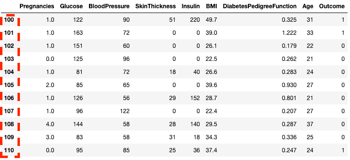

Isolating rows in pandas with .loc[]

df2.iloc[100:110]

Isolating rows in pandas with .iloc[]

You can also subset with .loc[] and .iloc[] by using a list instead of a range.

df2.loc[[100, 200, 300]]

Isolating rows using a list in pandas with .loc[]

df2.iloc[[100, 200, 300]]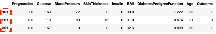

Isolating rows using a list in pandas with .iloc[]

You can also select specific columns along with rows. This is where .iloc[] is different from .loc[] – it requires column location and not column labels.

df2.loc[100:110, ['Pregnancies', 'Glucose', 'BloodPressure']]

Isolating columns in pandas with .loc[]

df2.iloc[100:110, :3]

Isolating columns with .iloc[]

For faster workflows, you can pass in the starting index of a row as a range.

df2.loc[760:, ['Pregnancies', 'Glucose', 'BloodPressure']]

Isolating columns and rows in pandas with .loc[]

df2.iloc[760:, :3]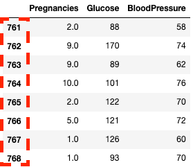

Isolating columns and rows in pandas with .iloc[]

You can update/modify certain values by using the assignment operator =

df2.loc[df['Age']==81, ['Age']] = 80

Conditional slicing (that fits certain conditions)

pandas lets you filter data by conditions over row/column values. For example, the below code selects the row where Blood Pressure is exactly 122. Here, we are isolating rows using the brackets [ ] as seen in previous sections. However, instead of inputting row indices or column names, we are inputting a condition where the column BloodPressure is equal to 122. We denote this condition using df.BloodPressure == 122.

df[df.BloodPressure == 122]

Isolating rows based on a condition in pandas 

The below example fetched all rows where Outcome is 1. Here df.Outcome selects that column, df.Outcome == 1 returns a Series of Boolean values determining which Outcomes are equal to 1, then [] takes a subset of df where that Boolean Series is True.

df[df.Outcome == 1]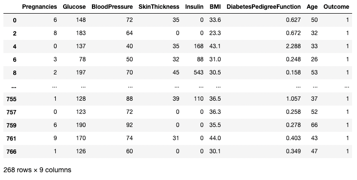

Isolating rows based on a condition in pandas 

You can use a > operator to draw comparisons. The below code fetches Pregnancies, Glucose, and BloodPressure for all records with BloodPressure greater than 100.

df.loc[df['BloodPressure'] > 100, ['Pregnancies', 'Glucose', 'BloodPressure']]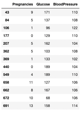

Isolating rows and columns based on a condition in pandas 

Cleaning data using pandas 

Data cleaning is one of the most common tasks in data science. pandas lets you preprocess data for any use, including but not limited to training machine learning and deep learning models. Let’s use the DataFrame df2 from earlier, having four missing values, to illustrate a few data cleaning use cases. As a reminder, here's how you can see how many missing values are in a DataFrame.

df2.isnull().sum()

Pregnancies                 4
Glucose                     0
BloodPressure               0
SkinThickness               0
Insulin                     0
BMI                         0
DiabetesPedigreeFunction    0
Age                         0
Outcome                     0
dtype: int64

Dealing with missing data technique #1: Dropping missing values

One way to deal with missing data is to drop it. This is particularly useful in cases where you have plenty of data and losing a small portion won’t impact the downstream analysis. You can use a .dropna() method as shown below. Here, we are saving the results from .dropna() into a DataFrame df3.

df3 = df2.copy()
df3 = df3.dropna()
df3.shape

(764, 9) # this is 4 rows less than df2

The axis argument lets you specify whether you are dropping rows, or columns, with missing values. The default axis removes the rows containing NaNs. Use axis = 1 to remove the columns with one or more NaN values. Also, notice how we are using the argument inplace=True which lets you skip saving the output of .dropna() into a new DataFrame.  

df3 = df2.copy()
df3.dropna(inplace=True, axis=1)
df3.head()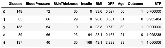

Dropping missing data in pandas

You can also drop both rows and columns with missing values by setting the how argument to 'all'

df3 = df2.copy()
df3.dropna(inplace=True, how='all')

Dealing with missing data technique #2: Replacing missing values

Instead of dropping, replacing missing values with a summary statistic or a specific value (depending on the use case) maybe the best way to go. For example, if there is one missing row from a temperature column denoting temperatures throughout the days of the week, replacing that missing value with the average temperature of that week may be more effective than dropping values completely. You can replace the missing data with the row, or column mean using the code below.

df3 = df2.copy()
# Get the mean of Pregnancies
mean_value = df3['Pregnancies'].mean()
# Fill missing values using .fillna()
df3 = df3.fillna(mean_value)

Dealing with Duplicate Data

Let's add some duplicates to the original data to learn how to eliminate duplicates in a DataFrame. Here, we are using the .concat() method to concatenate the rows of the df2 DataFrame to the df2 DataFrame, adding perfect duplicates of every row in df2. 

df3 = pd.concat([df2, df2])
df3.shape

(1536, 9)

You can remove all duplicate rows (default) from the DataFrame using .drop_duplicates() method.

df3 = df3.drop_duplicates()
df3.shape

(768, 9)

Renaming columns

A common data cleaning task is renaming columns. With the .rename() method, you can use columns as an argument to rename specific columns. The below code shows the dictionary for mapping old and new column names.

df3.rename(columns = {'DiabetesPedigreeFunction':'DPF'}, inplace = True)
df3.head()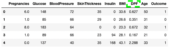

Renaming columns in pandas

You can also directly assign column names as a list to the DataFrame.

df3.columns = ['Glucose', 'BloodPressure', 'SkinThickness', 'Insulin', 'BMI', 'DPF', 'Age', 'Outcome', 'STF']
df3.head()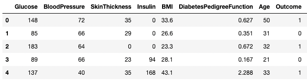

Renaming columns in pandas

For more on data cleaning, and for easier, more predictable data cleaning workflows, check out the following checklist, which provides you with a comprehensive set of common data cleaning tasks. 

Data analysis in pandas

The main value proposition of pandas lies in its quick data analysis functionality. In this section, we'll focus on a set of analysis techniques you can use in pandas.

Summary operators (mean, mode, median)

As you saw earlier, you can get the mean of each column value using the .mean() method.

df.mean()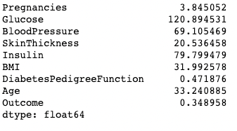

Printing the mean of columns in pandas

A mode can be computed similarly using the .mode() method. 

df.mode()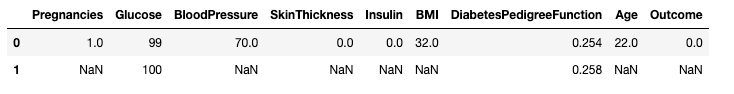

Printing the mode of columns in pandas

Similarly, the median of each column is computed with the .median() method

df.median()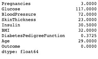

Printing the median of columns in pandas

Create new columns based on existing columns 

pandas provides fast and efficient computation by combining two or more columns like scalar variables. The below code divides each value in the column Glucose with the corresponding value in the Insulin column to compute a new column named Glucose_Insulin_Ratio.

df2['Glucose_Insulin_Ratio'] = df2['Glucose']/df2['Insulin']
df2.head()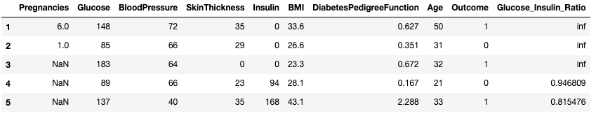

Create a new column from existing columns in pandas

Counting using .value_counts()

Often times you'll work with categorical values, and you'll want to count the number of observations each category has in a column. Category values can be counted using the .value_counts() methods. Here, for example, we are counting the number of observations where Outcome is diabetic (1) and the number of observations where the Outcome is non-diabetic (0).

df['Outcome'].value_counts()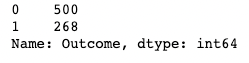

Using .value_counts() in pandas

Adding the normalize argument returns proportions instead of absolute counts.

df['Outcome'].value_counts(normalize=True)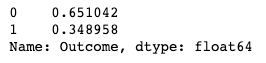

Using .value_counts() in pandas with normalization

Turn off automatic sorting of results using sort argument (True by default). The default sorting is based on the counts in descending order.

df['Outcome'].value_counts(sort=False)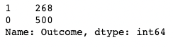

Using .value_counts() in pandas with sorting

You can also apply .value_counts() to a DataFrame object and specific columns within it instead of just a column. Here, for example, we are applying value_counts() on df with the subset argument, which takes in a list of columns. 

df.value_counts(subset=['Pregnancies', 'Outcome'])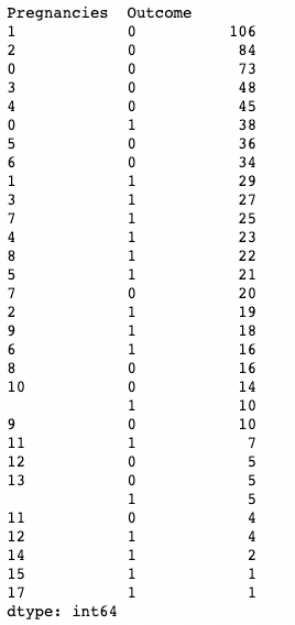

Using .value_counts() in pandas while subsetting columns

Aggregating data with .groupby() in pandas

pandas lets you aggregate values by grouping them by specific column values. You can do that by combining the .groupby() method with a summary method of your choice. The below code displays the mean of each of the numeric columns grouped by Outcome.

df.groupby('Outcome').mean()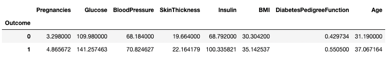

Aggregating data by one column in pandas

.groupby() enables grouping by more than one column by passing a list of column names, as shown below.

df.groupby(['Pregnancies', 'Outcome']).mean()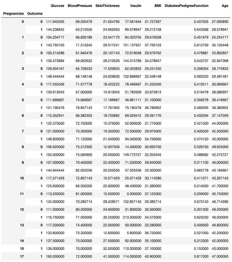

Aggregating data by two columns in pandas

Any summary method can be used alongside .groupby(), including .min(), .max(), .mean(), .median(), .sum(), .mode(), and more.

Pivot tables 

pandas also enables you to calculate summary statistics as pivot tables. This makes it easy to draw conclusions based on a combination of variables. The below code picks the rows as unique values of Pregnancies, the column values are the unique values of Outcome, and the cells contain the average value of BMI in the corresponding group.

For example, for Pregnancies = 5 and Outcome = 0, the average BMI turns out to be 31.1.

pd.pivot_table(df, values="BMI", index='Pregnancies', 
               columns=['Outcome'], aggfunc=np.me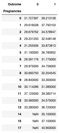an)

Aggregating data by pivoting with pandas

Data visualization in pandas

pandas provides convenience wrappers to Matplotlib plotting functions to make it easy to visualize your DataFrames. Below, you'll see how to do common data visualizations using pandas.

Line plots in pandas

pandas enables you to chart out the relationships among variables using line plots. Below is a line plot of BMI and Glucose versus the row index.

df[['BMI', 'Glucose']].plot.line()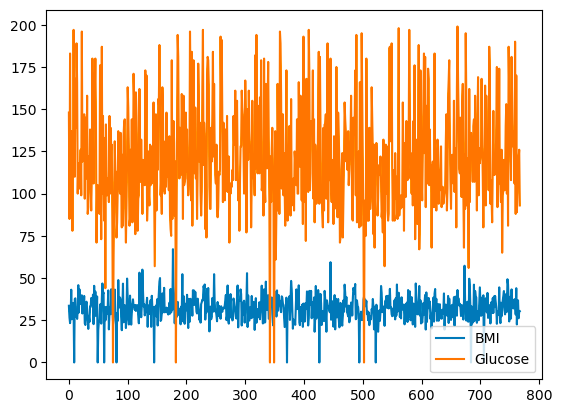

Basic line plot with pandas

You can select the choice of colors by using the color argument.

df[['BMI', 'Glucose']].plot.line(figsize=(20, 10), 
                                 color={"BMI": "red", "Glucose": "blue"})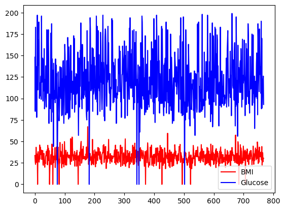

Basic line plot with pandas, with custom colors

All the columns of df can also be plotted on different scales and axes by using the subplots argument.

df.plot.line(subplots=True)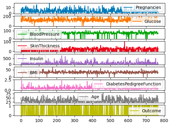

Subplots for line plots with pandas

Bar plots in pandas

For discrete columns, you can use a bar plot over the category counts to visualize their distribution. The variable Outcome with binary values is visualized below.

df['Outcome'].value_counts().plot.bar()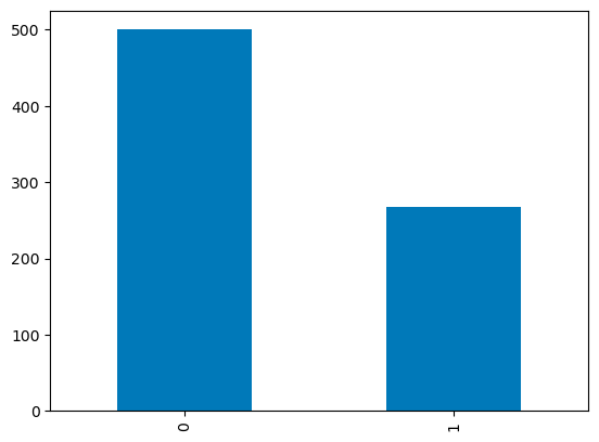

Barplots in pandas

Box plots in pandas

The quartile distribution of continuous variables can be visualized using a boxplot. The code below lets you create a boxplot with pandas.

df.boxplot(column=['BMI'], by='Outcome')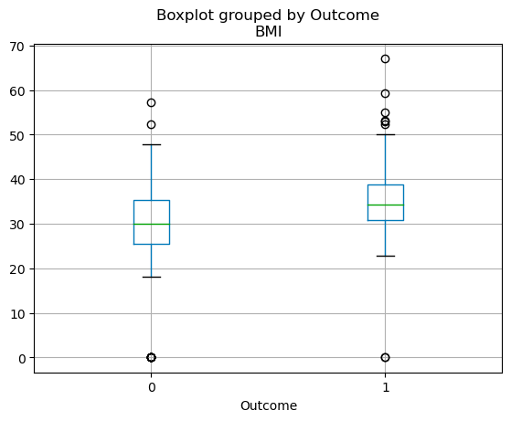

Boxplots in pandas

Learn more about pandas

The tutorial above scratches the surface of what's possible with pandas. Whether analyzing data, visualizing it, filtering, or aggregating it, pandas provides an incredibly rich feature set that lets you accelerate any data workflow. Moreover, by combining pandas with other data science packages, you'll be able to create interactive dashboards, create predictive models using machine learning, automate data workflows, and more. Check out the resources below to accelerate your pandas learning journey:

• [Cheat Sheets] A plethora of Python and pandas cheat sheets to reference throughout your learning 
• [Live trainings] Check out our free live-code-along sessions, many of which leverage pandas
• [More tutorials] Check out our remaining tutorials on pandas and the PyData ecosystem, including how to implement moving averages in pandas and using the pandas .apply() method