Fonction objectif : définition, exemples et optimisation

Chaque modèle d’apprentissage automatique que vous entraînez résout un problème d’optimisation — et ce que vous cherchez réellement à optimiser s’appelle la fonction objectif.

En termes simples, c’est une fonction mathématique qui mesure la « qualité » d’une solution. Elle prend un ensemble d’entrées et renvoie un score unique. L’objectif est toujours de trouver les valeurs qui maximisent ou minimisent ce score. Des programmes linéaires au deep learning, les fonctions objectif sont au cœur de tout. Une fois que vous avez compris leur mécanisme, vous les voyez partout.

Dans cet article, j’explique ce que sont les fonctions objectif, en quoi elles diffèrent des fonctions de perte et de coût, et comment elles sont utilisées en apprentissage automatique et en optimisation.

Vous cherchez une plongée en profondeur dans le deep learning toujours pertinente en 2026 ? Inscrivez-vous à notre cours Deep Learning in Python pour bâtir un portfolio PyTorch.

Qu’est-ce qu’une fonction objectif ?

Une fonction objectif est une fonction mathématique qui évalue la qualité d’une solution.

Vous lui fournissez un ensemble d’entrées — paramètres de modèle, variables de décision — et elle renvoie un nombre unique. Ce nombre indique la performance de votre solution actuelle. Plus ce nombre est élevé (ou faible), meilleure (ou moins bonne) est votre solution, selon que l’on maximise ou minimise.

Tant qu’on y est, parlons d’optimisation en général.

C’est le processus qui consiste à trouver les entrées qui poussent ce nombre dans la bonne direction. Si vous minimisez, vous voulez la valeur la plus faible possible. Si vous maximisez, vous voulez la plus élevée. Dans tous les cas, la fonction objectif est la mesure de référence.

Concrètement, pensez-y comme à un système de score. Chaque solution candidate obtient un score, et votre rôle est de trouver celle qui obtient le meilleur score.

Fonction objectif vs fonction de perte vs fonction de coût

Ces trois termes sont souvent employés de manière interchangeable — mais ils ne signifient pas exactement la même chose.

La fonction objectif est le terme le plus large. C’est toute fonction que vous cherchez à maximiser ou minimiser. Elle n’a pas besoin d’impliquer une erreur ou des prédictions — elle définit simplement ce que « mieux » signifie pour votre problème.

Une fonction de perte mesure l’erreur pour un seul exemple d’entraînement — l’écart entre la prédiction du modèle et la valeur réelle. L’erreur quadratique moyenne pour un point de données, par exemple, est une fonction de perte.

Une fonction de coût agrège la perte sur l’ensemble de votre jeu de données, généralement en la moyennant. C’est donc la fonction que vous minimisez réellement pendant l’entraînement — elle résume la performance du modèle sur tous les exemples, pas seulement un.

En pratique, la plupart des frameworks et articles de ML utilisent ces termes de manière souple. Vous verrez « loss » utilisé là où « cost » serait plus précis, et « objective » pour désigner les trois.

Ces distinctions comptent lorsque vous lisez des articles de recherche. Le contexte indique généralement lequel l’auteur vise réellement.

Pour une comparaison plus concrète, voir le tableau ci-dessous :

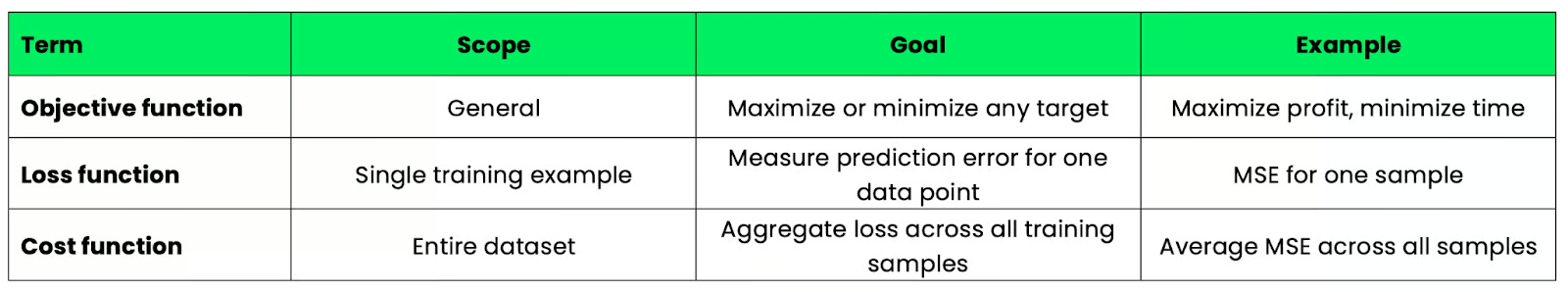
Tableau comparatif fonction objectif / perte / coût

Fonctions objectif en optimisation

Tout problème d’optimisation a un objectif et des limites.

La fonction objectif définit l’objectif — ce que vous cherchez à maximiser ou minimiser. Les contraintes définissent les limites — le périmètre dans lequel votre solution doit rester. Ensemble, elles cadrent le problème.

Prenons un exemple simple d’allocation de ressources.

Supposons que vous dirigiez une usine qui produit deux articles et que vous souhaitiez maximiser le profit. Votre fonction objectif traduit le profit total en fonction du nombre d’unités produites pour chaque produit. Vos contraintes capturent les limites — matières premières disponibles, heures machine, capacité de main-d’œuvre. La fonction objectif vous dit quoi optimiser et les contraintes ce avec quoi vous devez composer.

La programmation linéaire est l’un des cadres les plus courants pour cela. C’est une méthode qui optimise une fonction objectif linéaire sous contraintes linéaires. Elle est utilisée partout, de la logistique à la planification, de la supply chain à la finance. Les fondements mathématiques sont solides et les solveurs gèrent des problèmes avec des milliers de variables.

Il est important de noter que la fonction objectif ne change pas les contraintes — elle indique simplement au solveur ce qu’il doit viser. Si vous modifiez la fonction objectif, vous obtiendrez une solution complètement différente, même avec les mêmes contraintes.

Fonctions objectif en apprentissage automatique

En apprentissage automatique, la fonction objectif définit ce que votre modèle apprend réellement à faire.

À chaque entraînement, vous exécutez un algorithme d’optimisation (pensez à gradient descent, Adam, RMSProp) qui ajuste les paramètres du modèle pour minimiser ou maximiser la fonction objectif. Le modèle n’a aucune connaissance du problème métier. Il ne voit que le score que la fonction objectif lui attribue et cherche à l’améliorer à chaque mise à jour.

Votre choix de fonction objectif façonne donc le résultat. Il est pertinent d’en tester plusieurs pour voir celle qui fonctionne le mieux dans votre cas.

Erreur quadratique moyenne (régression)

L’erreur quadratique moyenne (MSE) est la fonction objectif par défaut pour les problèmes de régression. Elle mesure l’écart quadratique moyen entre les prédictions du modèle et les valeurs cibles réelles.

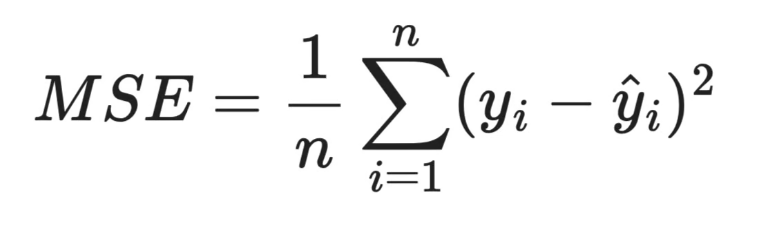
Formule de la MSE

Le fait de mettre les écarts au carré rend toutes les erreurs positives et pénalise davantage les grandes erreurs que les petites. Une prédiction erronée de 10 contribue 100 à la somme — pas seulement 10. La MSE est donc sensible aux valeurs aberrantes, ce qu’il faut surveiller avec des données réelles parfois « bruitées ».

import numpy as np

y_true = np.array([3.0, 5.0, 2.5, 7.0])
y_pred = np.array([2.8, 5.2, 2.0, 6.5])

mse = np.mean((y_true - y_pred) ** 2)
print(f"MSE: {mse:.4f}")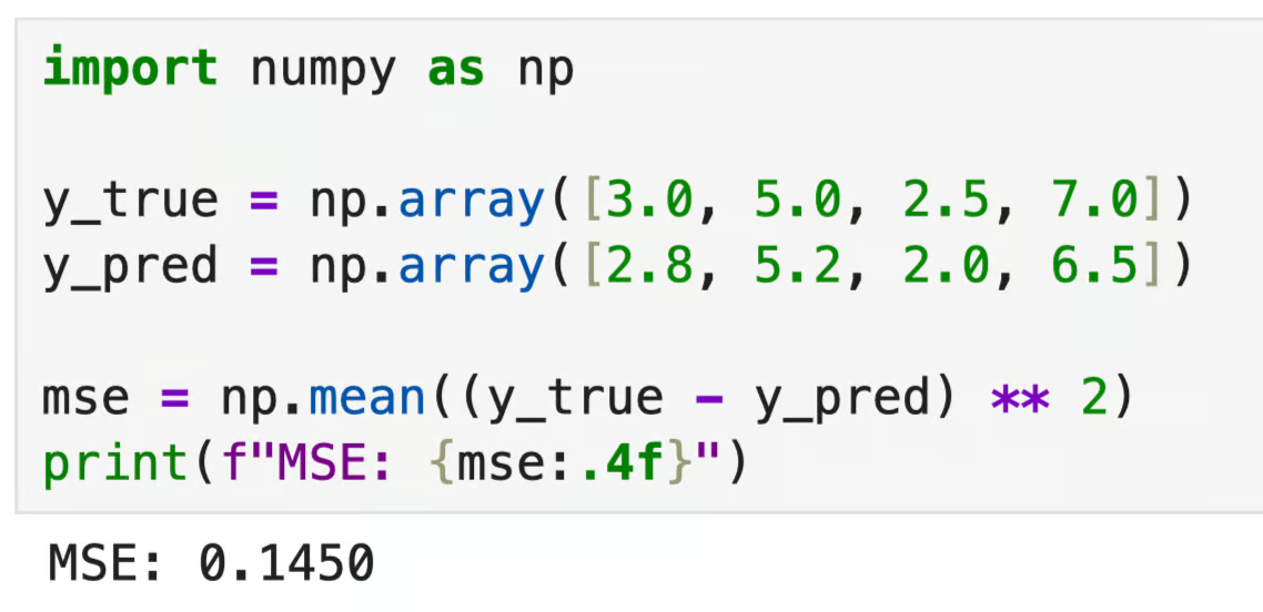

Sortie MSE

Perte d’entropie croisée (classification)

L’entropie croisée est la fonction objectif standard pour les problèmes de classification. Elle mesure l’écart entre la distribution de probabilités prédite par le modèle et la distribution de la vraie classe.

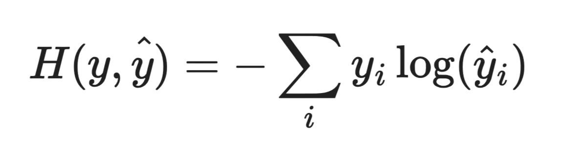
Fonction de perte d’entropie croisée

Si votre modèle attribue une probabilité élevée à la bonne classe, la perte est faible. S’il est confiant mais se trompe, la perte est élevée, et il est pénalisé. C’est ce qui pousse le modèle à prédire la bonne classe et à être confiant dans ses prédictions.

import numpy as np

# True labels (one-hot encoded)
y_true = np.array([1, 0, 0])

# Model's predicted probabilities
y_pred = np.array([0.7, 0.2, 0.1])

cross_entropy = -np.sum(y_true * np.log(y_pred))
print(f"Cross-Entropy Loss: {cross_entropy:.4f}")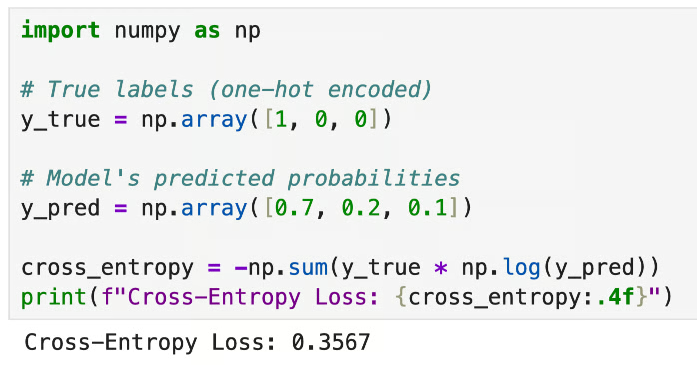

Sortie entropie croisée

Vraisemblance logarithmique

La log-vraisemblance est courante dans les modèles probabilistes et statistiques. La fonction consiste à maximiser la probabilité que les paramètres de votre modèle aient produit les données observées.

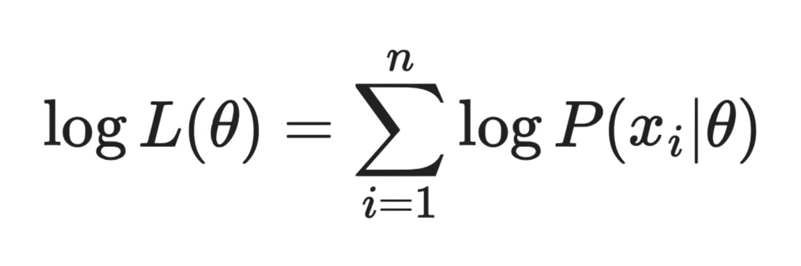
Formule de la log-vraisemblance

On travaille avec le logarithme de la vraisemblance plutôt qu’avec la vraisemblance elle-même, car il transforme un produit de probabilités en somme, bien plus simple à calculer et à optimiser.

En pratique, la plupart des frameworks minimisent la log-vraisemblance négative (NLL) au lieu de maximiser la log-vraisemblance. C’est équivalent — simplement inversé pour que la descente de gradient puisse fonctionner dessus.

import numpy as np
from scipy.stats import norm

# Observed data
data = np.array([1.2, 2.3, 1.8, 2.1, 1.9])

# Assumed model parameters
mu, sigma = 2.0, 0.5

# Compute negative log-likelihood
nll = -np.sum(norm.logpdf(data, loc=mu, scale=sigma))
print(f"Negative Log-Likelihood: {nll:.4f}")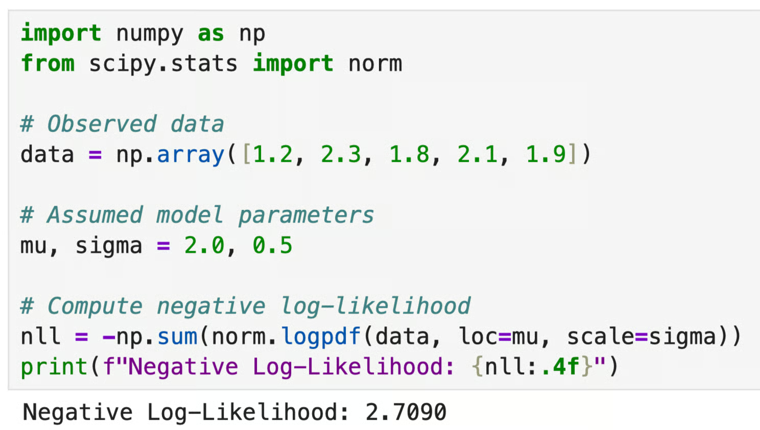

Sortie log-vraisemblance

L’entraînement est, au fond, de l’optimisation. Chaque passe avant calcule la valeur de la fonction objectif. Chaque rétropropagation calcule les gradients. Et chaque mise à jour des paramètres déplace le modèle dans la direction qui améliore le score.

Fonctions objectif convexes vs non convexes

Toutes les fonctions objectif ne se valent pas. Leur forme détermine la difficulté de l’optimisation et la fiabilité de la solution trouvée.

Fonctions objectif linéaires

Une fonction objectif linéaire décrit une relation en ligne droite entre les entrées et la sortie. Quand vous modifiez une entrée d’une quantité fixe, la sortie varie d’une quantité fixe.

Les fonctions linéaires sont utilisées en programmation linéaire, où l’objectif et les contraintes sont linéaires. Elles sont les plus faciles à optimiser : les solveurs trouvent de manière fiable l’optimum global, même pour de gros problèmes.

Fonctions objectif non linéaires

Une fonction objectif non linéaire a une relation plus complexe entre les entrées et la sortie. La plupart des problèmes réels — et presque tous les modèles de machine learning — entrent dans cette catégorie.

La MSE est non linéaire. L’entropie croisée est non linéaire. Les surfaces de perte des réseaux de neurones sont non linéaires. Cette complexité supplémentaire permet de capturer des relations riches dans les données, au prix d’une optimisation plus difficile.

Fonctions convexes versus non convexes

C’est là que les choses deviennent intéressantes.

Une fonction convexe a une forme en « bol ». Tout segment de droite tracé entre deux points de la courbe se situe au-dessus ou sur la courbe. Cela garantit que tout minimum local est aussi le minimum global — autrement dit, si votre optimiseur trouve un creux, c’est le bon.

Une fonction non convexe a une forme plus irrégulière — multiples vallées, plateaux et points selle. Les optimiseurs peuvent se retrouver coincés dans un minimum local, une vallée qui ressemble au fond mais ne l’est pas. Les réseaux de neurones profonds ont des surfaces de perte très non convexes ; c’est pourquoi leur entraînement exige un réglage soigné des taux d’apprentissage, des optimiseurs et de l’initialisation.

Les problèmes convexes se résolvent exactement, et les problèmes non convexes s’approximent. La qualité de votre solution dépend de votre stratégie d’optimisation.

Pour les esprits visuels, voici une comparaison entre fonctions objectif linéaires, non linéaires, convexes et non convexes :

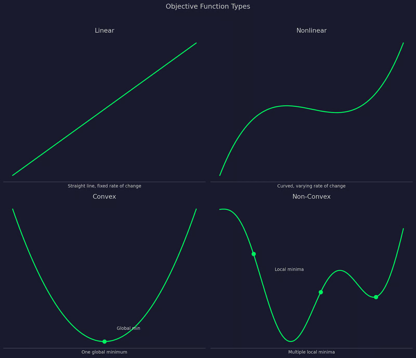
Comparaison des types de fonctions objectif

Comment optimiser les fonctions objectif

Une fois la fonction objectif définie, il faut un moyen de la minimiser ou de la maximiser. C’est le rôle des algorithmes d’optimisation.

L’approche la plus courante est la descente de gradient. L’idée : calculer le gradient de la fonction objectif par rapport aux paramètres du modèle, puis faire un petit pas dans la direction qui réduit la valeur. On répète jusqu’à ce que la valeur cesse de s’améliorer.

Le gradient n’est rien d’autre que la dérivée de la fonction objectif.

Il vous donne la pente à votre position actuelle et la direction de la « montée ». Pour minimiser la fonction, vous vous déplacez en sens opposé. Pour la maximiser, vous allez dans le même sens.

Le processus est itératif : pour atteindre la solution, vous effectuez une série de petites mises à jour qui rapprochent les paramètres de l’optimum. La taille de chaque pas est contrôlée par le taux d’apprentissage. Trop grand : vous risquez de dépasser l’optimum ; trop petit : l’entraînement s’éternise.

En pratique, la plupart des frameworks de ML utilisent des variantes plus rapides et plus stables que la version de base :

• Stochastic Gradient Descent (SGD) calcule le gradient sur un seul exemple aléatoire par pas, au lieu de tout le jeu de données
• Descente de gradient par mini-lots utilise un petit lot d’exemples à chaque pas — un compromis entre SGD et le lot complet
• Adam adapte le taux d’apprentissage pour chaque paramètre, ce qui facilite le réglage

La fonction objectif doit être différentiable, ou au moins en grande partie différentiable, pour que les méthodes basées sur le gradient fonctionnent. Pas de dérivée = pas de gradient, et l’optimiseur n’a plus de direction à suivre. C’est un point clé à retenir.

Exemple de fonction objectif

Rendons cela concret avec une simple régression linéaire.

Supposons que vous prédisez le prix des maisons à partir de la surface habitable. Vous disposez d’un jeu de données avec des prix connus et vous souhaitez ajuster une droite qui minimise l’erreur de prédiction. Votre fonction objectif est l’erreur quadratique moyenne (MSE) dont vous connaissez déjà la formule.

Les entrées sont les paramètres du modèle — la pente et l’ordonnée à l’origine de la droite. La sortie est un nombre unique — l’erreur quadratique moyenne sur toutes les prédictions. Ici, plus c’est bas, mieux c’est.

Voici à quoi pourrait ressembler une implémentation Python :

import numpy as np

np.random.seed(42)

# Generate some fake housing data
square_footage = np.random.uniform(500, 3000, 100)
true_price = 150 * square_footage + 50000 + np.random.normal(0, 15000, 100)

def predict(x, slope, intercept):
    return slope * x + intercept

def mse(y_true, y_pred):
    return np.mean((y_true - y_pred) ** 2)

# Try two different parameter sets
slope_a, intercept_a = 150, 50000  # good fit
slope_b, intercept_b = 80, 100000  # bad fit

pred_a = predict(square_footage, slope_a, intercept_a)
pred_b = predict(square_footage, slope_b, intercept_b)

print(f"MSE (good fit):  {mse(true_price, pred_a):,.2f}")
print(f"MSE (poor fit):  {mse(true_price, pred_b):,.2f}")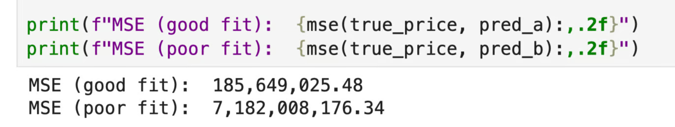

MSE : bon vs mauvais ajustement

Le premier jeu de paramètres produit une MSE bien plus faible, ce qui signifie un meilleur ajustement aux données. C’est exactement ce dont l’optimiseur se sert pour décider de la direction à prendre.

Pour les profils visuels, considérez l’image suivante :

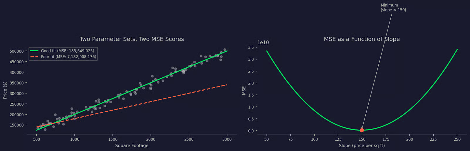
Exemple de MSE

Vous voyez les deux ajustements par rapport aux données et la surface de la MSE sur un éventail de valeurs de pente — autrement dit, la fonction objectif elle-même.

Le graphique de gauche montre comment les deux jeux de paramètres s’ajustent aux données. Celui de droite montre la surface de la MSE en fonction de la pente — la fonction objectif sous forme de courbe, avec un minimum net que l’optimiseur cherche à atteindre. Chaque pas de la descente de gradient progresse le long de cette courbe vers ce minimum.

Contraintes et fonctions objectif

La fonction objectif indique ce qu’il faut optimiser. Les contraintes indiquent ce que vous êtes autorisé à faire.

Dans la plupart des problèmes réels, vous ne pouvez pas maximiser ou minimiser à votre guise. Vous devez respecter des limites, comme un budget, une fenêtre temporelle ou une capacité physique. Ces limites sont des contraintes, et elles définissent l’ensemble des solutions valides dans lequel l’optimiseur peut chercher.

Prenons un exemple industriel.

Vous souhaitez maximiser le profit sur deux lignes de produits. Sans contraintes, la réponse est de produire autant que possible. Mais vous disposez de 500 heures machine et de 1 000 unités de matière première. Voilà vos contraintes. La fonction objectif reste la même (maximiser le profit), mais l’optimiseur ne peut explorer que la région autorisée par ces contraintes.

Si vous modifiez les contraintes, la solution optimale change aussi, même si la fonction objectif ne change pas.

Cette structure — une fonction objectif assortie de contraintes — est le fondement de l’optimisation sous contraintes. C’est ainsi que fonctionne la programmation linéaire, l’optimisation de portefeuille, et la formulation de nombreux problèmes de planification réels.

Conclusion

Tout problème d’optimisation — qu’il s’agisse d’entraîner un réseau de neurones, d’allouer des ressources ou d’ajuster un modèle de régression — se ramène à une chose : une fonction que vous cherchez à minimiser ou maximiser.

La fonction objectif, c’est cette fonction. Elle définit ce que « mieux » signifie, guide chaque mise à jour de paramètres et détermine ce que votre modèle apprend réellement. Si vous la choisissez bien, votre modèle pourra résoudre le problème que vous avez. Si vous vous trompez, il résoudra un autre problème — souvent sans signal d’alerte évident.

Choisir la bonne fonction objectif est une décision de conception en data science, car elle façonne tout le reste. En tant que praticien, n’hésitez pas à expérimenter — il existe de nombreuses fonctions objectif parmi lesquelles choisir.

Vous ne savez pas par où commencer ? Nos cours Model Validation in Python et Hyperparameter Tuning in Python sont d’excellents points de départ pour les data scientists débutants à intermédiaires.