Pernahkah Anda menjalankan uji t, mendapatkan p-value yang rapi, lalu menyadari bahwa Anda belum mengecek apakah data Anda berdistribusi normal?

Uji statistik tidak memberi tahu saat asumsinya dilanggar. Mereka hanya melaporkan nilainya. Masalahnya, uji seperti uji t dan ANOVA mengasumsikan data Anda mengikuti distribusi normal. Jika tidak, Anda membangun kesimpulan di atas fondasi yang rapuh.

Uji normalitas memberi Anda cara untuk memverifikasi asumsi tersebut. Ada metode visual dan statistik untuk melakukannya, dan mengetahui mana yang digunakan - serta cara membaca hasilnya - memungkinkan Anda dengan percaya diri mendukung hasil Anda.

Dalam artikel ini, saya akan memandu Anda melalui metode visual dan statistik paling umum untuk memeriksa normalitas, menunjukkan cara menjalankannya di Python dan R, serta menjelaskan apa yang harus dilakukan saat data Anda tidak lolos uji.

Apa Itu Distribusi Normal dalam Praktik

Anda mungkin pernah melihat kurva lonceng sebelumnya - namun inilah maknanya bagi data Anda.

Distribusi normal adalah pola di mana sebagian besar nilai mengelompok di sekitar pusat, dan makin sedikit nilai saat Anda bergerak menjauh ke kedua sisi. Saat dipetakan, Anda mendapatkan kurva berbentuk lonceng yang simetris. Sisi kiri mencerminkan sisi kanan.

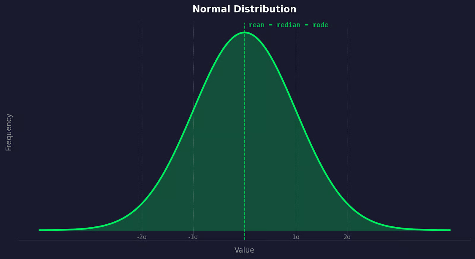
Plot distribusi normal

Yang membuat distribusi normal unik adalah mean, median, dan modus semuanya berada pada titik yang sama - pusat lonceng. Tidak ada kemencengan ke kiri atau kanan. Dengan kata lain, datanya seimbang.

Hal ini sering muncul dalam data pengukuran dunia nyata. Tinggi badan manusia, pembacaan tekanan darah, toleransi manufaktur, nilai ujian - semuanya cenderung mengikuti distribusi normal saat Anda mengumpulkan sampel yang cukup banyak. Variasi alami dalam sistem biologis dan fisik cenderung menghasilkan bentuk ini.

Namun, tidak semua data berperilaku demikian. Data pendapatan menceng ke kanan. Waktu respons situs web memiliki ekor panjang.

Di dunia nyata, hal-hal bisa jadi sangat buruk jika Anda berasumsi normalitas tanpa mengeceknya.

Mengapa Pengujian Normalitas Penting

Masalah tidak memeriksa normalitas adalah bahwa sebagian besar uji statistik umum - uji t, ANOVA - adalah uji parametrik.

Artinya, uji tersebut dibangun di atas asumsi tentang distribusi data Anda. Normalitas adalah salah satunya. Saat asumsi itu patah, matematika uji tersebut ikut bermasalah. Anda tetap akan mendapat hasil uji, tetapi hasil itu bisa menyesatkan Anda ke kesimpulan yang salah.

Uji parametrik bekerja dengan membuat asumsi matematis tentang populasi asal sampel Anda. Saat asumsi tersebut terpenuhi, uji ini berguna dan akurat. Saat tidak, p-value Anda menjadi tidak dapat diandalkan dan Anda tidak bisa membuat kesimpulan yang tepat.

Di sinilah uji nonparametrik berperan.

Uji seperti Mann-Whitney U atau Kruskal-Wallis tidak mengasumsikan normalitas - uji ini bekerja dengan peringkat alih-alih nilai mentah. Uji ini lebih fleksibel, namun juga cenderung kurang berguna saat data Anda normal. Jadi beralih ke sana tanpa perlu bukanlah jawabannya.

Masalah sebenarnya yang sering dilakukan pemula data science adalah sama sekali melewatkan pemeriksaan.

Pengujian normalitas hanya membutuhkan beberapa baris kode. Tidak mengujinya berarti Anda entah mempercayai data Anda begitu saja - atau tidak memikirkannya sama sekali.

Metode Visual untuk Memeriksa Normalitas

Sebelum menjalankan uji formal apa pun, plot data Anda. Visual akan banyak memberi tahu tentang apa yang Anda hadapi.

Histogram

Histogram menunjukkan bentuk distribusi Anda.

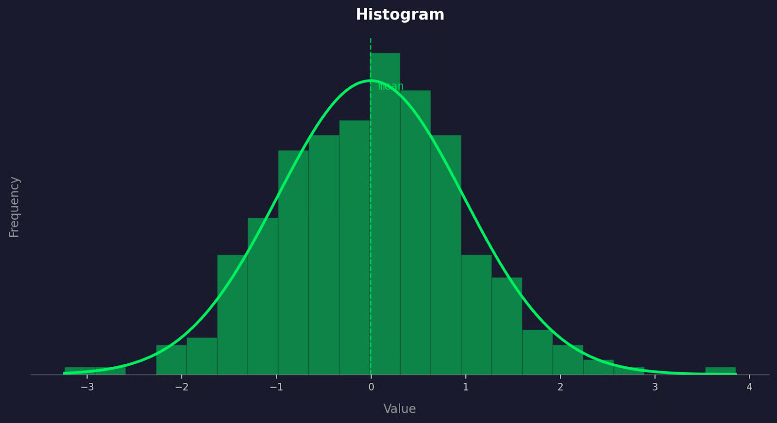
Contoh histogram

Jika data Anda berdistribusi normal, histogram akan terlihat seperti kurva lonceng - tinggi di tengah, meruncing simetris di kedua sisi. Yang perlu Anda perhatikan adalah kemencengan (skewness): ekor panjang yang tertarik ke kanan berarti kemencengan positif, ekor yang tertarik ke kiri berarti kemencengan negatif. Keduanya menandakan data Anda mungkin tidak normal.

Masalah pada histogram adalah bentuknya bergantung pada ukuran bin:

• Bin terlalu sedikit dan distribusi terlihat datar
• Terlalu banyak dan terlihat bergerigi

Selalu coba beberapa ukuran bin sebelum menarik kesimpulan.

Q-Q plot

Sebuah Q-Q plot (quantile-quantile plot) membandingkan kuantil data Anda dengan kuantil dari distribusi normal teoretis.

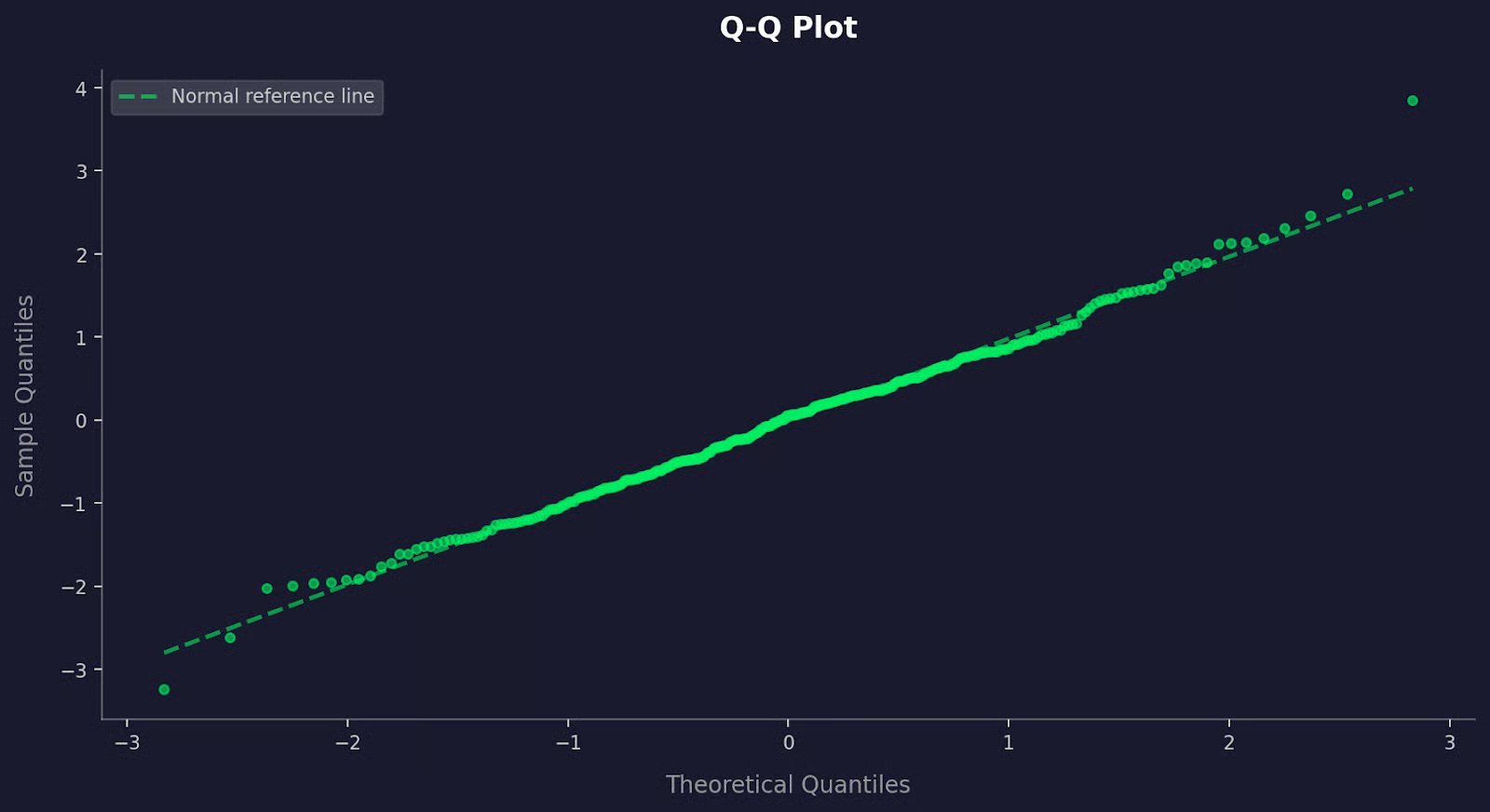
Contoh Q-Q plot

Jika data Anda normal, titik-titiknya jatuh di sepanjang garis diagonal lurus. Penyimpangan dari garis itu memberi tahu di mana normalitas tidak terpenuhi. Titik yang melengkung ke atas di bagian ujung menunjukkan ekor berat. Kurva berbentuk S menandakan kemencengan.

Q-Q plot lebih presisi daripada histogram untuk mendeteksi penyimpangan halus dari normalitas - terutama pada bagian ekor, yang sering luput pada histogram.

Box plot

Box plot menampilkan median, sebaran, dan pencilan dalam satu tampilan.

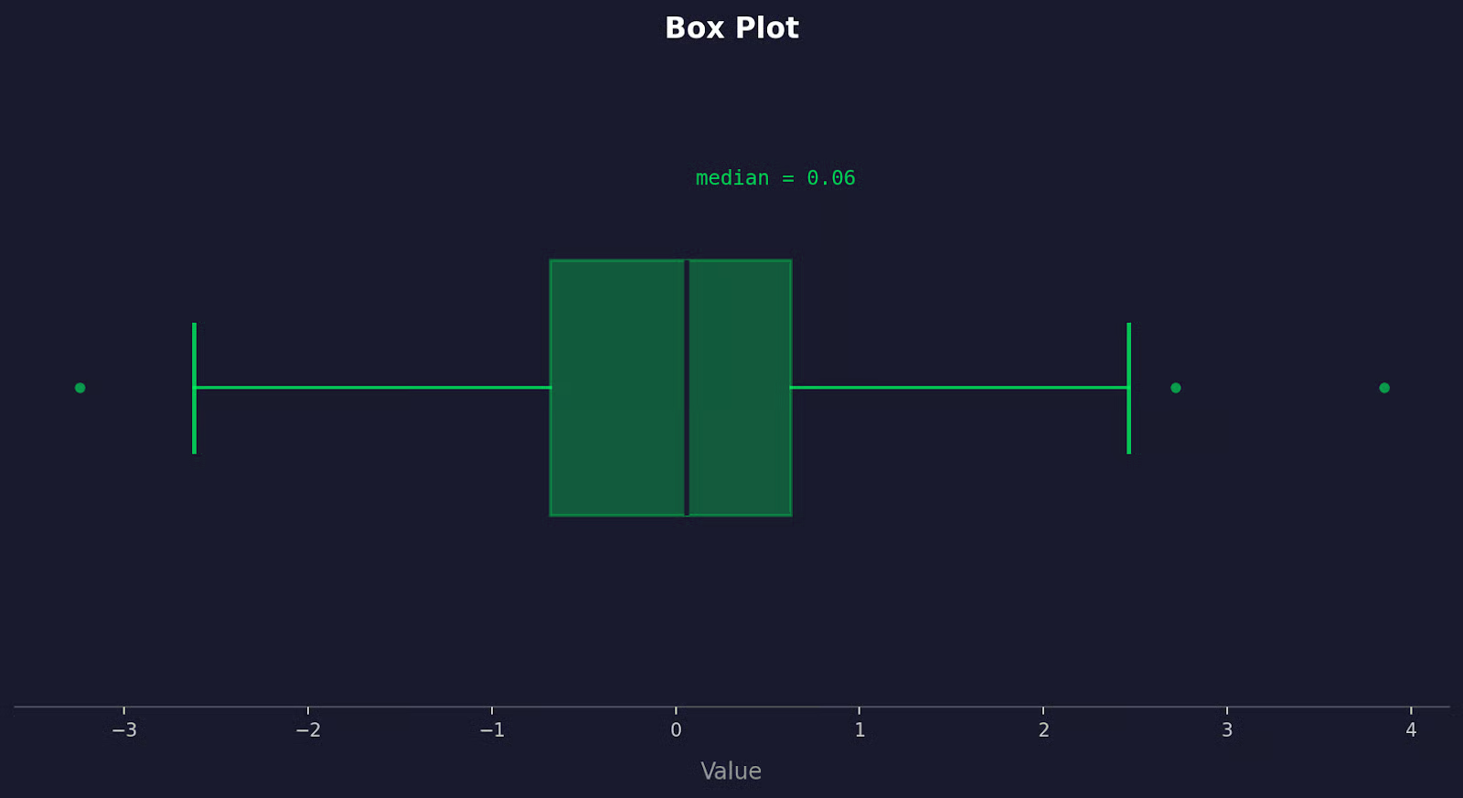
Contoh box plot

Dataset yang berdistribusi normal menghasilkan box plot dengan median yang berada kira-kira di tengah kotak, dan whisker memanjang dengan panjang yang kurang lebih sama di kedua sisi. Jika median tidak di tengah, atau salah satu whisker jauh lebih panjang dari yang lain, itu adalah kemencengan. Titik di luar whisker adalah pencilan.

Masalah umum pada visual adalah sifatnya yang subjektif. Dua orang bisa melihat histogram yang sama dan tidak sepakat. Gunakan untuk mendapat gambaran awal, lalu konfirmasi dengan uji formal.

Uji Normalitas yang Umum dalam Statistik

Tidak ada satu uji normalitas yang paling baik di setiap situasi. Pilihan yang tepat bergantung pada ukuran sampel dan apa yang ingin Anda deteksi.

Uji Shapiro-Wilk

Uji Shapiro-Wilk adalah pilihan utama untuk sampel kecil hingga menengah, umumnya hingga beberapa ratus pengamatan.

Uji ini mengukur seberapa dekat data Anda cocok dengan distribusi normal dengan membandingkan nilai yang diamati dengan apa yang diharapkan jika data normal. Uji ini banyak digunakan, dipahami dengan baik, dan tersedia di setiap pustaka statistik utama. Bagi sebagian besar analis, ini adalah uji pertama yang patut dicoba.

Keterbatasan utamanya adalah menjadi terlalu sensitif pada ukuran sampel besar. Cenderung menandai penyimpangan kecil yang secara praktis tidak bermakna sebagai signifikan secara statistik.

Uji Kolmogorov-Smirnov

Uji Kolmogorov-Smirnov (KS) membandingkan distribusi kumulatif sampel Anda dengan distribusi teoretis - dalam hal ini, normal.

Uji ini lebih umum daripada Shapiro-Wilk dan dapat menguji terhadap distribusi apa pun, bukan hanya normal. KS kurang bertenaga dibanding Shapiro-Wilk untuk pengujian normalitas, artinya lebih kecil kemungkinannya menangkap penyimpangan halus. Uji ini juga mengharuskan Anda menentukan parameter distribusi di awal, yang memperkenalkan bias jika Anda mengestimasinya dari data yang sama.

Gunakan saat Anda butuh pemeriksaan cepat serbaguna - bukan sebagai uji normalitas utama.

Uji Anderson-Darling

Uji Anderson-Darling adalah variasi dari uji KS, namun dengan satu perbedaan kunci: memberi bobot lebih besar pada bagian ekor distribusi.

Ini membuatnya lebih baik dalam menangkap penyimpangan yang muncul pada ekstrem - ekor berat, pencilan, atau perilaku non-normal yang mungkin luput dari uji KS. Jika kasus penggunaan Anda sensitif terhadap perilaku ekor, Anderson-Darling adalah pilihan yang baik.

Uji D'Agostino-Pearson

Uji D'Agostino-Pearson mengambil pendekatan yang berbeda.

Alih-alih langsung membandingkan distribusi, uji ini mengukur dua properti data Anda: kemencengan (asimetrinya) dan kurtosis (seberapa berat atau ringannya ekor).

Keduanya digabungkan menjadi satu statistik uji. Ini membuatnya bagus untuk mengidentifikasi mengapa data Anda mungkin tidak normal - bukan hanya apakah normal atau tidak. Bekerja paling baik pada sampel besar, saat estimasi kemencengan dan kurtosis andal.

Uji Jarque-Bera

Uji Jarque-Bera juga menggunakan kemencengan dan kurtosis, mirip dengan D'Agostino-Pearson.

Uji ini umum dalam ekonometrika dan analisis deret waktu. Seperti D'Agostino-Pearson, uji ini membutuhkan sampel yang cukup besar untuk menghasilkan hasil yang andal. Dengan sampel kecil, uji ini kurang dapat diandalkan. Jika Anda bekerja dalam konteks keuangan atau ekonomi, Anda mungkin sering melihat uji ini.

Sebagai penutup, mulailah dengan Shapiro-Wilk untuk sampel kecil dan padukan dengan Q-Q plot. Gunakan Anderson-Darling saat perilaku ekor penting, dan D'Agostino-Pearson saat Anda ingin memahami sifat penyimpangannya.

Cara Menginterpretasikan Hasil Uji Normalitas

Setiap uji normalitas adalah uji hipotesis.

Hipotesis nol dalam uji normalitas mana pun adalah bahwa data Anda berdistribusi normal. Uji kemudian menanyakan: mengingat apa yang kita lihat pada data, seberapa besar kemungkinan hipotesis nol ini benar?

Jawabannya kembali sebagai p-value:

• p > 0,05 - Anda tidak memiliki cukup bukti untuk menolak normalitas. Asumsikan data normal dan lanjutkan dengan uji parametrik
• p < 0,05 - data berbeda dari normalitas cukup besar hingga terdeteksi secara statistik. Tolak asumsi normalitas

Terdengar sederhana, tetapi banyak orang keliru di sini.

p-value yang rendah tidak memberi tahu seberapa tidak normal data Anda - hanya bahwa ada perbedaan yang terdeteksi. Dengan sampel besar, uji normalitas menjadi sangat sensitif. Uji akan menandai penyimpangan yang begitu kecil hingga tidak berdampak nyata pada analisis Anda.

Masalah sebaliknya juga ada. Dengan sampel kecil, bahkan data yang terlihat menceng bisa menghasilkan p > 0,05 karena uji tidak memiliki daya yang cukup untuk mendeteksi penyimpangan.

Signifikansi statistik dan signifikansi praktis bukanlah hal yang sama.

p-value memberi tahu Anda apakah ada penyimpangan dari normalitas. Ini tidak memberi tahu apakah penyimpangan tersebut penting bagi analisis spesifik Anda. Selalu padukan hasil uji dengan Q-Q plot - jika titik-titik mengikuti garis dengan erat, data Anda mungkin cukup normal, terlepas dari apa kata p-value.

Uji Normalitas di Python

Modul scipy.stats di Python memiliki semua yang Anda butuhkan untuk menjalankan uji normalitas hanya dalam beberapa baris kode.

Untuk semua contoh di bawah, saya akan menggunakan dataset yang sama - 100 sampel yang diambil dari distribusi normal - sehingga Anda bisa menjalankan kode dan mengikutinya.

import numpy as np
from scipy import stats

np.random.seed(42)
data = np.random.normal(loc=0, scale=1, size=100)

Uji Shapiro-Wilk

Gunakan shapiro() sebagai pemeriksaan pertama, terutama pada dataset yang lebih kecil.

stat, p_value = stats.shapiro(data)
print(f"Statistic: {stat:.4f}, p-value: {p_value:.4f}")

Berikut yang Anda dapatkan:

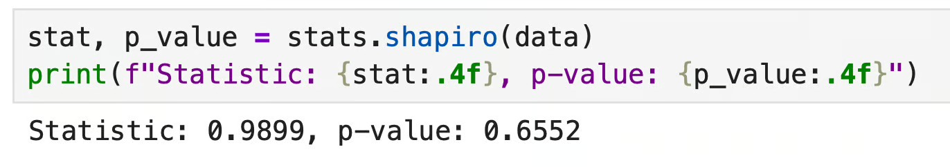
Keluaran uji Shapiro-Wilk di Python

p-value jauh di atas 0,05, jadi kita tidak menolak normalitas. Datanya terlihat normal - masuk akal, karena kita menghasilkannya dari distribusi normal.

Uji Kolmogorov-Smirnov

kstest() membandingkan sampel Anda dengan distribusi bernama. Untuk normalitas, berikan "norm" bersama mean dan simpangan baku sampel.

stat, p_value = stats.kstest(data, 'norm', args=(data.mean(), data.std()))
print(f"Statistic: {stat:.4f}, p-value: {p_value:.4f}")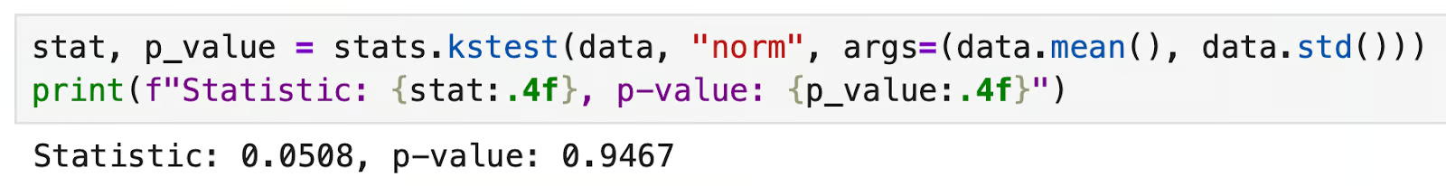

Keluaran uji Kolmogorov-Smirnov di Python

Lagi-lagi, p > 0,05 - tidak ada bukti menentang normalitas.

Dengan uji ini di Python, selalu berikan mean dan simpangan baku secara eksplisit melalui args. Jika dilewati, kstest() akan default ke normal standar (mean=0, sd=1), yang akan memberi hasil tidak andal kecuali data Anda sudah distandardisasi.

Uji D'Agostino-Pearson

normaltest() menguji normalitas dengan memeriksa gabungan kemencengan dan kurtosis. Bekerja paling baik pada sampel yang lebih besar.

stat, p_value = stats.normaltest(data)
print(f"Statistic: {stat:.4f}, p-value: {p_value:.4f}")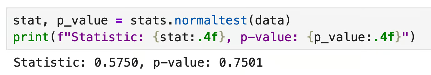

Keluaran uji D'Agostino-Pearson di Python

p > 0,05 lagi. Data lolos ketiga uji di sini, namun itu memang diharapkan - saya membangkitkannya agar normal. Dalam praktik, Anda sering melihat uji-uji ini tidak sepakat, terutama di sekitar batas 0,05. Saat itu terjadi, kembali ke Q-Q plot Anda untuk membuat keputusan.

Uji Normalitas di R

R memiliki fungsi bawaan untuk pengujian normalitas. Tidak membutuhkan paket tambahan untuk hal-hal dasar.

Seperti pada contoh Python, saya akan menggunakan dataset yang sama: 100 sampel dari distribusi normal.

set.seed(42)
data <- rnorm(100, mean = 0, sd = 1)

Uji Shapiro-Wilk

shapiro.test() adalah andalan untuk sampel kecil hingga menengah. Cukup berikan vektor data Anda:

shapiro.test(data)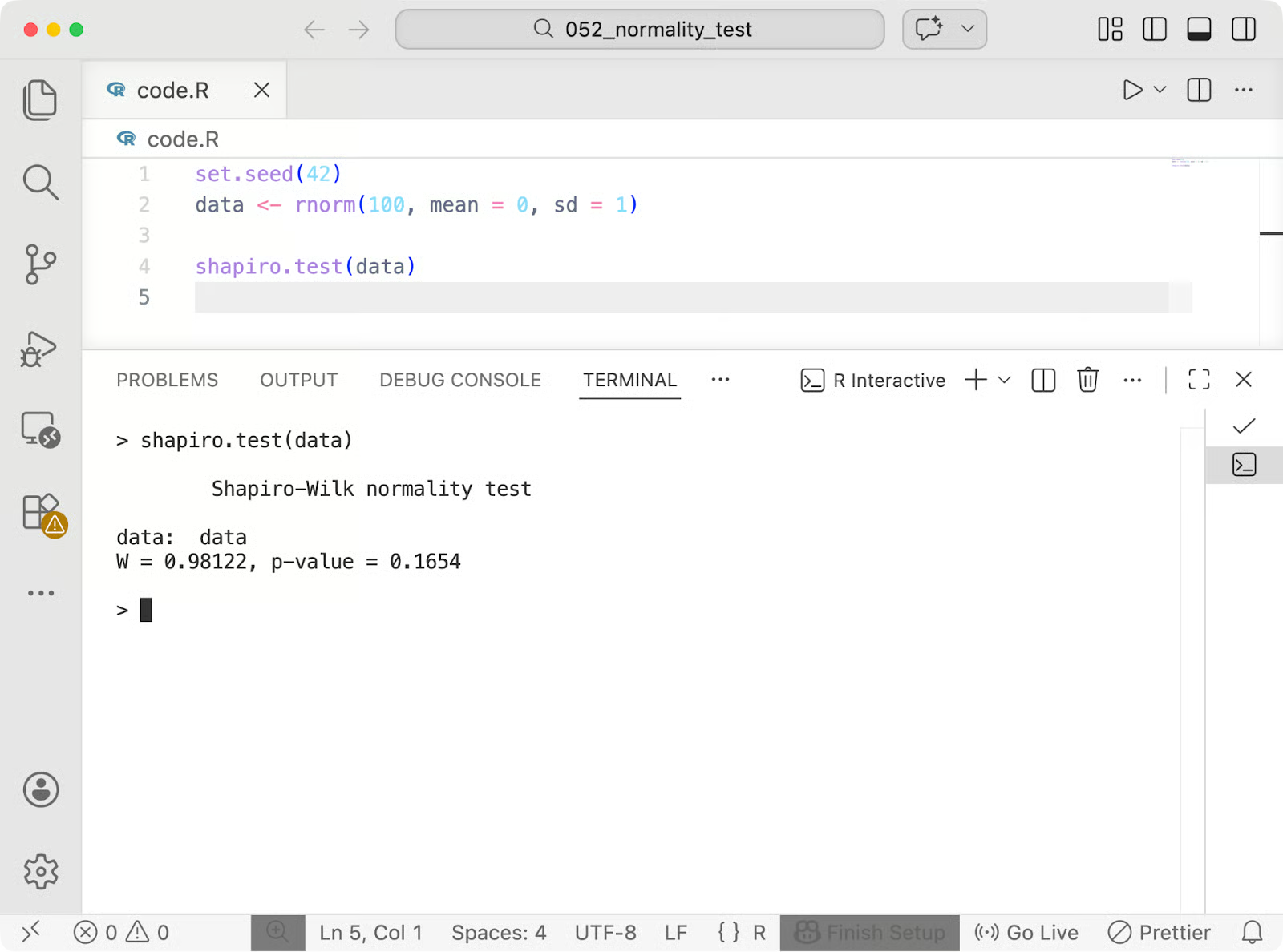

Keluaran uji Shapiro-Wilk di R

p > 0,05 - tidak ada bukti menentang normalitas. Statistik W berkisar dari 0 hingga 1, di mana nilai yang mendekati 1 menunjukkan data sangat mengikuti distribusi normal.

Uji Kolmogorov-Smirnov

ks.test() membandingkan sampel Anda dengan distribusi teoretis. Untuk normalitas, tentukan "pnorm" dan berikan mean serta simpangan baku sampel.

ks.test(data, "pnorm", mean(data), sd(data))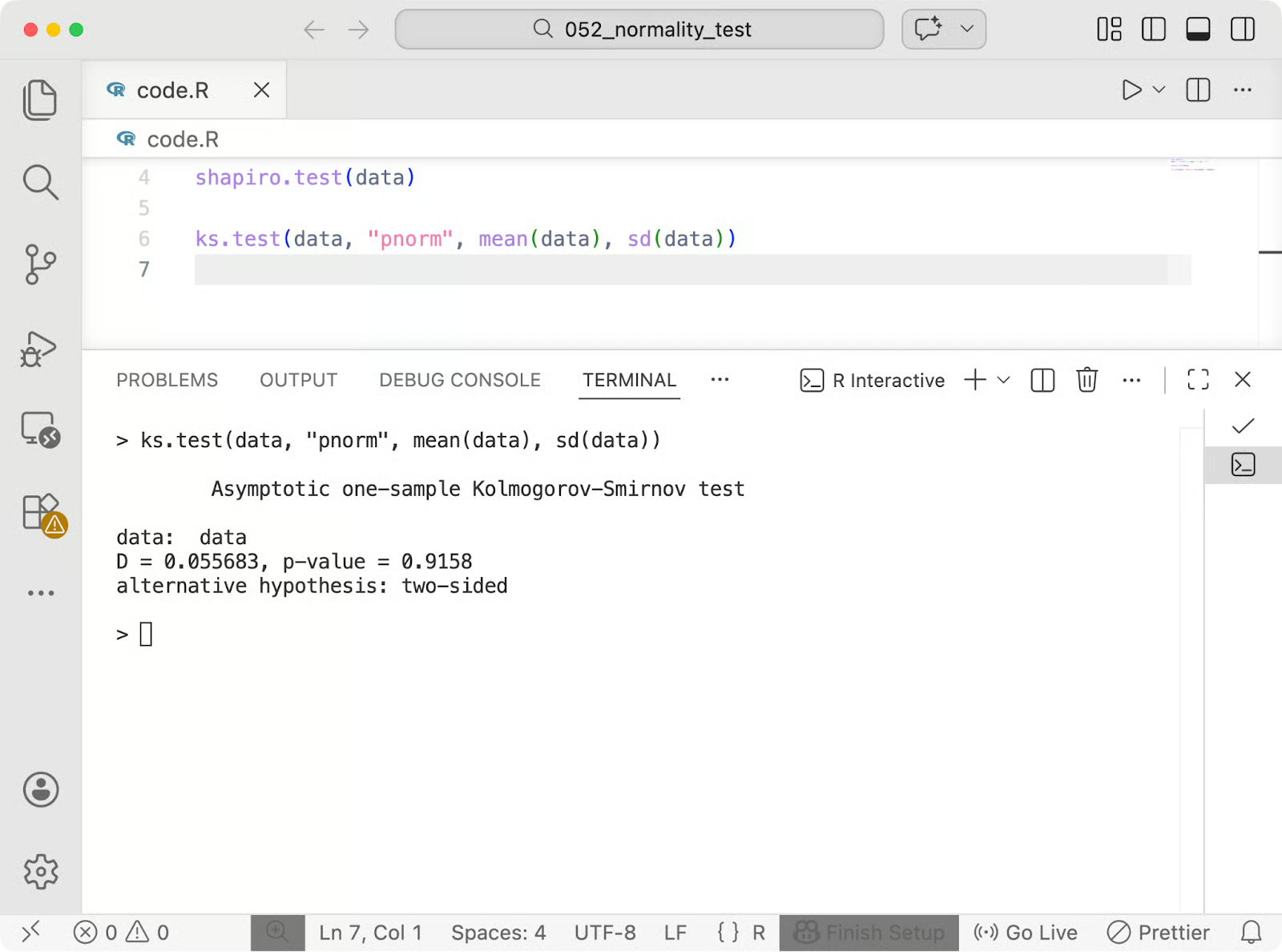

Keluaran uji Kolmogorov-Smirnov di R

p > 0,05 lagi. Uji ini di R memiliki catatan yang sama seperti di Python: selalu berikan mean(data) dan sd(data). Melewatkannya akan default ke normal standar, yang membelokkan hasil kecuali data Anda sudah distandardisasi.

Q-Q plot

Fungsi bawaan R qqnorm() dan qqline() memberi Anda Q-Q plot dalam dua baris kode.

qqnorm(data, main = "Q-Q Plot")
qqline(data, col = "steelblue", lwd = 2)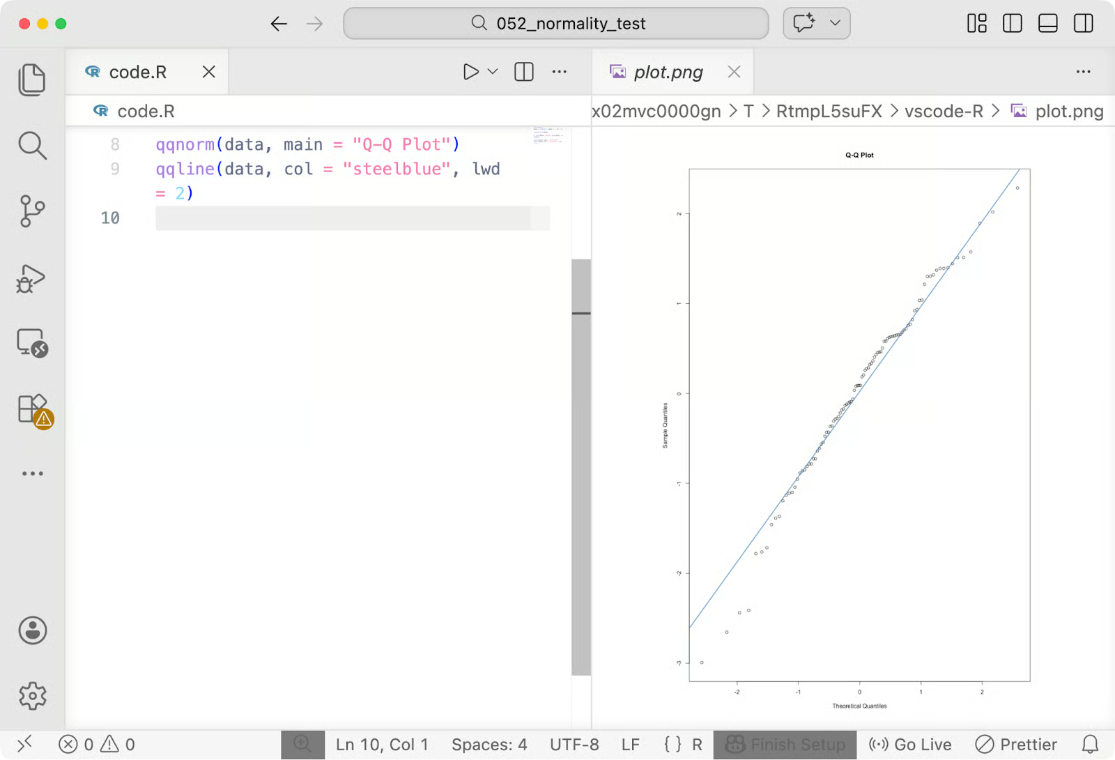

Q-Q plot di R

qqnorm() memplot kuantil sampel Anda terhadap kuantil normal teoretis. qqline() menggambar garis referensi. Titik-titik yang mengikuti garis tersebut dengan erat berarti data Anda berperilaku normal. Penyimpangan di bagian ujung menandakan masalah ekor yang layak diselidiki.

Apa yang Harus Dilakukan Jika Data Tidak Normal

Jika data Anda gagal dalam uji normalitas, Anda memiliki beberapa opsi yang solid.

Transformasi data

Terkadang solusinya adalah mentransformasi data agar berperilaku normal, lalu jalankan uji asli Anda pada nilai yang telah ditransformasi.

Transformasi log adalah pilihan paling umum. Bekerja baik pada data menceng ke kanan - misalnya pendapatan, waktu respons, atau pengukuran biologis yang memiliki ekor panjang di sisi kanan. Fungsinya di Python adalah np.log(data), dan padanannya di R adalah log(data).

Transformasi akar kuadrat adalah opsi yang lebih ringan untuk kemencengan sedang, dan berguna saat data Anda mengandung nol (karena Anda tidak bisa mengambil log dari nol). Gunakan np.sqrt(data) di Python atau sqrt(data) di R.

Setelah ditransformasi, jalankan kembali uji normalitas. Jika data yang ditransformasi lolos, lanjutkan dengan uji parametrik Anda - ingatlah untuk menafsirkan hasil dalam skala yang telah ditransformasi.

Gunakan uji nonparametrik

Jika transformasi tidak berhasil atau tidak masuk akal untuk data Anda, beralihlah ke uji nonparametrik. Uji ini tidak mengasumsikan normalitas - uji ini memberi peringkat data alih-alih bekerja dengan nilai mentah.

• Uji Mann-Whitney U adalah alternatif nonparametrik untuk uji t dua sampel independen. Gunakan saat Anda membandingkan dua kelompok
• Uji Kruskal-Wallis adalah versi nonparametrik dari ANOVA satu arah. Gunakan saat Anda membandingkan tiga kelompok atau lebih

Keduanya tersedia di scipy.stats (mannwhitneyu() dan kruskal()) dan di paket dasar R (wilcox.test() dan kruskal.test()).

Andalkan ukuran sampel besar

Dengan sampel yang cukup besar, Anda sering kali dapat mengabaikan kekhawatiran tentang normalitas.

Teorema limit pusat menyatakan bahwa seiring bertambahnya ukuran sampel, distribusi sampling dari mean mendekati normal - terlepas dari bagaimana distribusi data aslinya. Dalam praktik, ini berarti uji parametrik cenderung andal dengan sampel besar bahkan saat data dasarnya tidak benar-benar normal.

Kesalahan Umum Saat Menguji Normalitas

Pengujian normalitas itu mudah - Anda telah melihat bahwa ini hanya membutuhkan satu baris kode. Namun tetap saja, ada beberapa cara untuk keliru.

Berikut beberapa kesalahan umum yang sering dilakukan pemula data science:

• Hanya mengandalkan p-value: p-value memberi tahu apakah penyimpangan dari normalitas terdeteksi, bukan seberapa besar penyimpangan itu atau apakah itu penting. Menganggap p > 0,05 sebagai lampu hijau dan p < 0,05 sebagai lampu merah terlalu kaku. Selalu padukan hasil uji Anda dengan Q-Q plot
• Mengabaikan efek ukuran sampel: Dengan sampel kecil, uji normalitas bisa melewatkan penyimpangan nyata dan mengembalikan p > 0,05 meski data Anda terlihat menceng. Dengan sampel besar, uji menjadi sangat sensitif hingga menandai penyimpangan kecil yang tidak bermakna sebagai signifikan. Ukuran sampel dapat mengubah makna p-value
• Terlalu sering menguji normalitas: Tidak setiap analisis membutuhkan uji normalitas formal. Jika Anda sedang eksplorasi, histogram dan Q-Q plot biasanya cukup
• Salah menafsirkan penyimpangan kecil: Data dunia nyata hampir tidak pernah benar-benar normal. Penyimpangan kecil dari garis referensi pada Q-Q plot, atau p-value yang sedikit di bawah 0,05, tidak berarti data Anda jauh dari normal. Pertanyaannya adalah apakah cukup normal untuk uji yang Anda jalankan

Jadi sebagai kesimpulan, pengujian normalitas hanyalah satu pemeriksaan terhadap data Anda. Gunakan sebagai salah satu masukan, bukan kata akhir.

Kapan Anda Bisa Melewatkan Uji Normalitas

Uji normalitas tidak selalu diperlukan. Jika Anda dikejar tenggat, mengetahui kapan bisa melewatkannya dapat menghemat waktu tanpa memengaruhi hasil.

Dataset besar

Saat Anda memiliki sampel besar, teorema limit pusat menjamin bahwa distribusi sampling dari mean kira-kira normal, apa pun bentuk data mentah Anda. Uji parametrik umumnya andal dalam situasi ini, jadi menjalankan uji normalitas formal memberi nilai tambah yang kecil.

Beberapa metode statistik juga tangguh terhadap ketidaknormalan. Teknik seperti regresi linear cenderung tetap baik saat ukuran sampel memadai, dan pelanggarannya tidak ekstrem. (Regresi linear tetap mengasumsikan normalitas pada residual.)

Analisis eksploratori

Saat Anda memindai data untuk mencari pola, membangun intuisi, atau memutuskan variabel mana yang akan ditelusuri lebih jauh, histogram cepat atau Q-Q plot sudah cukup. Uji formal untuk analisis konfirmatori - saat kesimpulan Anda perlu dapat dipertanggungjawabkan.

Ingat bahwa uji normalitas ada untuk melindungi Anda dari penarikan kesimpulan yang salah. Jika Anda berada dalam konteks di mana kesimpulan yang salah tidak membawa konsekuensi nyata, atau metode Anda tidak bergantung pada normalitas, uji tersebut bersifat opsional.

Kesimpulan

Pengujian normalitas bertujuan untuk memeriksa apakah asumsi Anda cukup terpenuhi agar hasil dapat dipercaya.

Tidak ada dataset yang sempurna normal. Tujuannya adalah memahami bagaimana data Anda berperilaku dan memilih metode yang sesuai. Q-Q plot memberi tahu di mana penyimpangan berada. Uji formal memberi tahu apakah penyimpangan itu terdeteksi secara statistik. Jika digabungkan, keduanya memberi gambaran yang lebih jelas daripada salah satunya saja.

Uji yang tepat bergantung pada konteks Anda. Gunakan Shapiro-Wilk untuk sampel kecil, Anderson-Darling saat bagian ekor penting, alternatif nonparametrik saat normalitas tidak bisa diasumsikan. Dan terkadang - dengan sampel besar atau metode yang tangguh - tidak perlu uji sama sekali.

Apakah Anda merasa konsep p-value membingungkan? Baca artikel kami Hypothesis Testing Made Easy untuk memastikan Anda menafsirkannya dengan benar.