Central Limit Theorem: A Key Concept in Statistics Explained

If we take lots of random samples from pretty much any type of data distribution, something surprising happens. The average of those samples starts to look like a normal distribution – that familiar bell-shaped curve. That’s the central limit theorem (CLT) in a nutshell.

It’s a big deal in probability and statistics because it means we can make accurate predictions and draw conclusions about whole populations, even when only looking at small samples.

What makes the CLT extra useful is that it works even if the original data isn’t normally distributed. Let’s explore this in detail and see how we can calculate it. 

What Is the Central Limit Theorem?

The central limit theorem, or CLT, is an idea in statistics that says that if we take a bunch of random samples from any population and look at the averages of those samples, those averages will start to form a normal, bell-shaped curve even if the original population doesn’t look normal at all.

This connects to the law of large numbers, which tells us that as we collect more data, our sample average gets closer and closer to the true average of the whole population. The CLT takes that a step further — it tells us that the sample average becomes more accurate and that the pattern of those averages becomes predictable. Our Intro to Statistics course has practice exercises to get you familiar with the relationship and differences between the CLT and the law of large numbers, if you want to explore this part further.

A great way to see this in action is by rolling a die. If we roll it just once, we get a random number between 1 and 6. But after enough rolls, the average will settle around 3.5 (the true average value of a fair die). Do this repeatedly, and the distribution of those averages starts to look like a normal curve.

Central Limit Theorem Formula

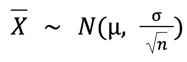
Here’s the basic formula for the central limit theorem:

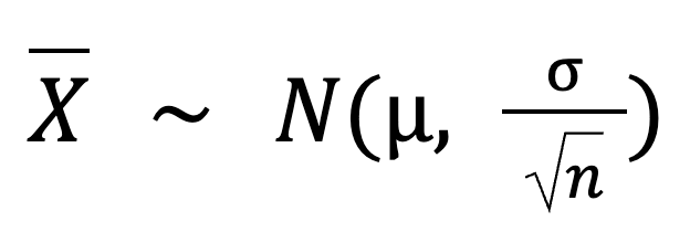
In this formula:

• X is the sampling distribution of the sample mean, which follows a normal distribution. 

• N is the normal distribution.

• 𝜇 is the population mean.

• σ is the population standard deviation.

• n is the sample size.

As the sample size gets bigger, the standard deviation of the sampling distribution gets smaller. The more data we collect, the more tightly our sample means will cluster around the true population mean.

Central Limit Theorem Conditions

Now, for the central limit theorem to work the way we expect, there are a few conditions to consider:

• Sufficiently large sample size: The sample size has to be large enough. A sample size of 30 or more is usually considered good. But if the population we’re sampling from is skewed or has many outliers, we may need a bigger sample to see that nice, bell-shaped curve show up.
• Independent and Identically Distributed (i.i.d.) samples: The samples we take need to be independent and identically distributed(i.i.d.). This means each sample is chosen randomly and comes from the same population. If that’s not true, then the results may not be reliable.
• Finite population variance: The population we’re sampling must have a finite variance. If the data comes from a distribution with infinite variance, like the Cauchy distribution, the CLT won’t apply to those.

Central Limit Theorem Examples

Let’s say we want to know how many cups of coffee are sold per day at a local coffee shop. Over the years, the number of cups sold each day may follow a distribution similar to the one I'm including here. Most days, they sell between 80 and 120 cups. But on busy days like holidays or special events, they sell 150 or even 180 cups. The data is a bit skewed (uneven) in this case.

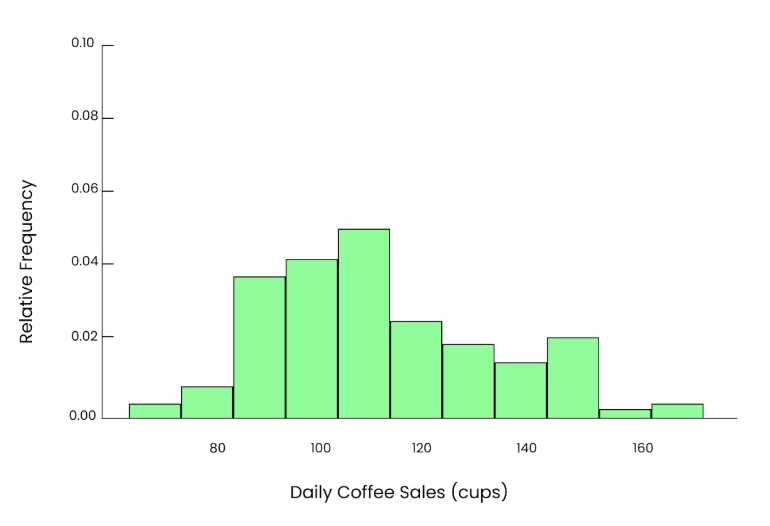
Uneven graph. Image by Author.

Let’s say we take a small sample. We randomly pick 5 days from the year and look at how many cups were sold on those days. 

95, 102, 85, 110, 120

The mean we get from this sample is:

Mean = 95+102+85+110+1205 = 102.4 cups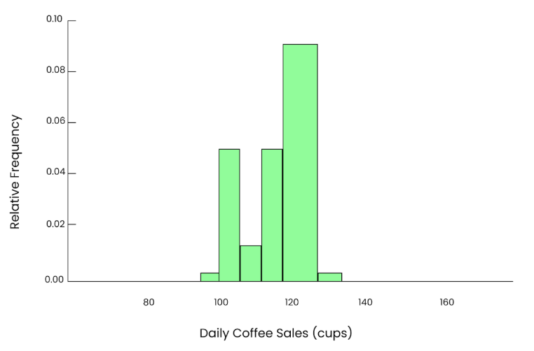

Graph of 5 cups. Image by Author.

That gives us one estimate of the population mean, but since the sample is small, it may not be exact. If we repeat this process 10 times, randomly pick 5 days each time, calculate the mean, and write down the results. The 10 sample means would be: 

97.6, 105.8, 93.4, 110.2, 99.0, 102.4, 101.2, 107.5, 96.3, 94.1

If we plot these values in a histogram, we’ll see a rough bell shape, but it may still look uneven. And the spread of these means is smaller than the spread in the population. 

Graph of 10 cups. Image by Author.

Now, let’s take a bigger sample. This time, we randomly select 50 days and calculate the mean number of cups sold:

98, 104, 87, 112, 105, 100, 108, 95, 102, 106,
92, 115, 97, 101, 109, 103, 96, 110, 104, 98,
100, 102, 89, 107, 94, 111, 108, 90, 100, 103,
106, 99, 96, 112, 105, 97, 100, 104, 93, 110,
107, 102, 95, 101, 99, 103, 109, 98, 94, 100

When we calculate the mean of this sample, we get:

Mean = 101.2 cups

This estimate is much closer to the population mean of 100, and because our sample size is larger, it’s a more precise estimate.

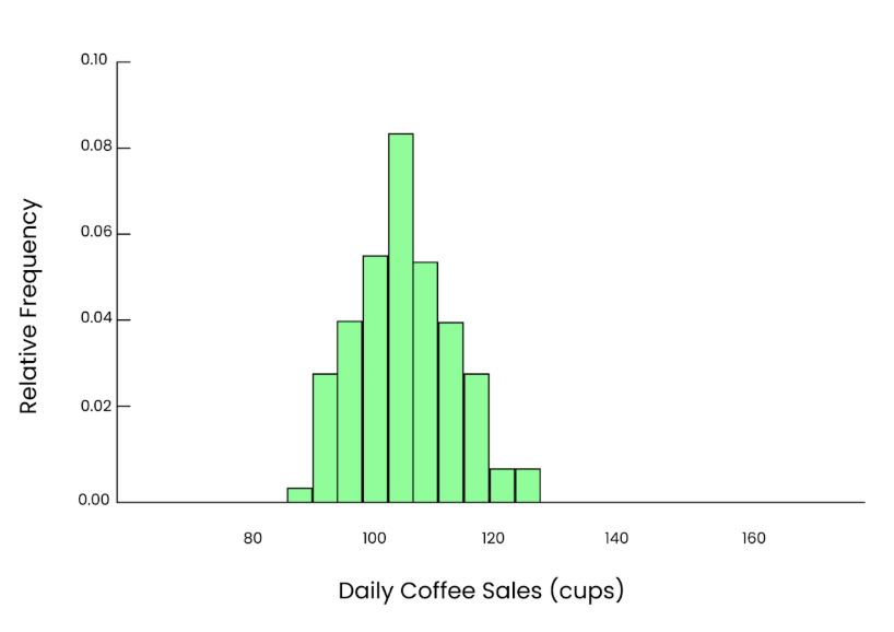
If we repeat this process many times, each time randomly selecting 50 days, calculating the mean, and plotting those means in a histogram, even though the original data was skewed, we’ll see an apparent, smooth bell-shaped curve. So, that’s the power of the central limit theorem.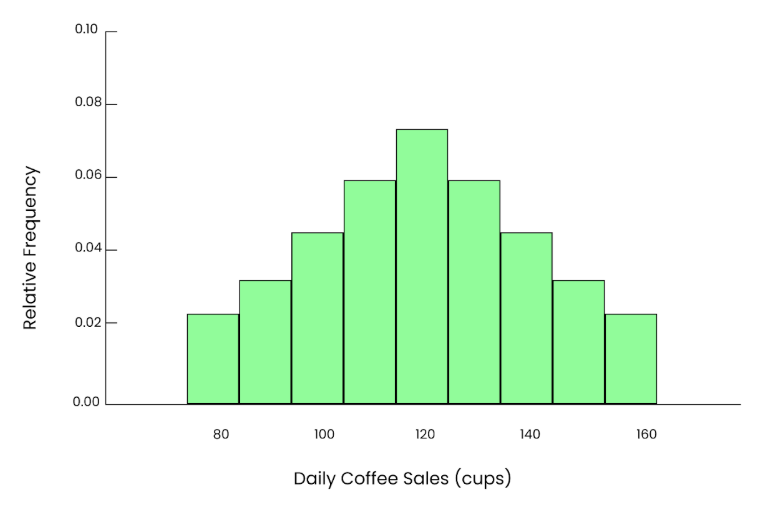

Even graph. Image by Author.

We can even calculate that spread using this formula:

Here:

• µ(population mean) = 100

• σ (population standard deviation) = 15

• n (sample size) = 50

So, the standard deviation of our sample means is:

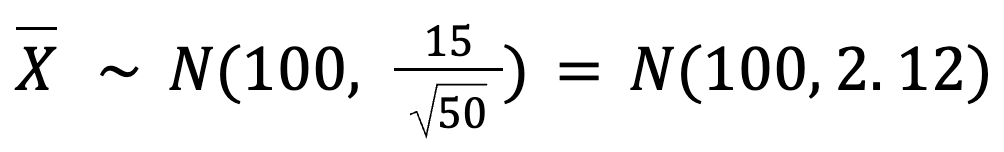
This tells us that the sample means will be very close to 100 cups with just a small variation (around 2.12 cups).

Why the Central Limit Theorem Matters

Now we know data in the real world can be weird and unpredictable. But the central limit theorem gives us a reliable way to understand what’s going on and make better choices based on it. Let’s understand its importance in more detail. 

Statistical inference

In statistics, the central limit theorem is the reason why parametric tests like t-tests, ANOVA, and regression work the way they do. These tests are based on the idea that sample data comes from a population with fixed characteristics.

Without the central limit theorem, we wouldn’t be able to rely on those tests. And because of this theorem, parametric tests are often more potent than non-parametric ones, which don’t make assumptions about the data’s distribution.

Industry applications

It also shows up in a lot of real-world situations. In finance, analysts use it to estimate average stock returns based on past performance. In polling and surveys, it makes predictions about the entire population by collecting a sample of responses. In machine learning and big data, we use it where models are trained on samples. For example, a movie app may use a sample of user activity to build its recommendation system.

Central Limit Theorem Calculator

Standard deviation is a number that tells us how spread the values are from the average. When we look at sample means (the averages from different samples), we want to know how much those averages vary. For that, we can use this formula:

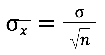
This tells us that when we divide the population standard deviation by the square root of the sample size, we get the standard deviation of the sampling distribution. As the sample size gets bigger, the overall value gets smaller. 

Let’s look at a quick example:

You can see that the mean stays the same, but the standard deviation keeps shrinking. This shows that the bigger the sample, the more accurate and consistent it is.

The Central Limit Theorem in Data Science

In data science, we usually deal with samples, not whole populations. The CLT helps us understand how those sample results behave and it tells us that if we take enough samples, their averages will start to look like a normal distribution, even if the original data is anything but.

This has some big real-world perks too. In machine learning, we often use techniques like bootstrapping to estimate values. Thanks to the CLT, we can be confident that those estimates are accurate.

It’s also a key player in A/B testing. When a company tries out two versions of a webpage or feature, the CLT helps us figure out whether the results are meaningful or random noise.

Even in reinforcement learning, where systems learn by trial and error, the CLT irons out the chaos. As more data rolls in, the averages become more stable, which helps the system learn faster and better.

Finally, you’ll also spot the CLT in hypothesis testing and time series analysis. It helps data scientists test ideas and track trends with more confidence.

Final Thoughts

The central limit theorem may sound technical if you’re new to stats, but it’s a big reason we can do smart things with data. It turns randomness into something we can understand and trust. In fact, it’s one of the building blocks of statistical modeling and a must-know for anyone who works with data. 

If you want to explore more, read up on the law of large numbers and probability distributions — they all tie together.