The Standard Normal Distribution: What It Is and Why It Matters

You may notice the bell curve, which goes by many names, like the normal distribution or the Gaussian distribution, practically everywhere, especially if you have an eye for statistics or data science. It feels like but is not an accident of nature: It turns out a lot of what we measure is the result of many small factors added together, hinting at the presence of an underlying additive model.

By transforming any normal distribution into a special form called the standard normal distribution, we can create a distribution that is especially useful in specific contexts, such as computing probabilities, making statistical inferences, and applying statistical tests. By the end of this article, you will be clear about what the standard normal distribution is, why we take the extra step of standardizing it, and how all this relates to variability, probability, and hypothesis testing. By the end, I hope you will also enroll in our Introduction to Statistics in R course or our Statistical Inference in R skill track to keep building on the ideas in this article.

What is the Standard Normal Distribution?

The standard normal distribution is a specific form of the normal distribution where the mean is zero, and the standard deviation is one. We should also say the distribution is symmetric and that the probabilities of certain values decrease symmetrically as you move away from the center.

"Standard Normal Distribution" Image by Dall-E

Let’s look a little more closely into the mathematical aspects of the standard normal distribution.

The PDF of the standard normal distribution 

If you are not familiar with the idea of a probability density function (PDF), know that it describes how probabilities are distributed over the possible values of a continuous random variable. Every continuous probability distribution, like the exponential distribution, the t-distribution, or the Cauchy distribution, has its own probability density function that defines the curve. The PDF of the standard normal distribution is defined here: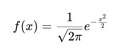

This function ensures that the area under the curve integrates to 1. If you look at the equation and plug in different values of x, you get the height of the curve at those points. In the equation:

• x represents any real number and is the input variable for the function. It appears in the exponent of the function, which is −x²/2. This controls the shape of the curve.
• Since x² is always non-negative, and there is a negative sign in front, the exponent is always negative or zero.
• In the specific case where x=0, the exponent is largest, making f(x) reach its peak. 
• If x moves away from 0 in either the positive or negative direction, x² increases, making the exponent more negative. A more negative exponent results in a smaller function value, meaning, together with the other things we said, the f(x) decreases symmetrically on both sides of x=0.
• The base of the exponent, which is Euler’s number, ensures the rapid decay of the function as x moves further from zero in either direction.
• The constant 1/√(2π) ensures the total area under the curve equals 1.

The CDF of the standard normal distribution

Unlike the PDF, which gives the relative likelihood of different values, the CDF tells you the probability that a variable is less than or equal to a given value. Just like the PDF, every continuous probability distribution has its own CDF.

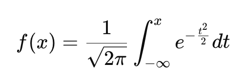
This equation is a bit more complicated, but we can work through it:

• The integral means that instead of giving the height of the curve at x, the CDF tells us the total probability from −∞ to x.
• When x→−∞, the CDF approaches 0.
• When x=0 the CDF is 0.5, since the distribution is symmetric and half the probability lies to the left of zero.
• As x→∞, the CDF approaches 1.

Why We Care About the Standard Normal Distribution 

Our guide on the Gaussian distribution has some good ideas on when you might want to conform your data to a normal distribution. But sometimes, you might want to change your data into a standard normal specifically. Here are some common reasons why:

The standard normal is used in hypothesis testing

A standard normal distribution makes our data more comparable and usable with certain statistical methods. By converting data into Z-scores, we can compare observations across different normal distributions. In particular, it forms the basis of Z-tests, which we use when we want to determine if a sample mean significantly differs from a population mean. 

The t-test, on the other hand, uses the sample standard deviation as an estimate of the population standard deviation, which is why it relies on the t-distribution, which has heavier tails than the standard normal distribution. Read our tutorial T-test vs. Z-test: When to Use Each, which talks about things like population and sample variance. 

The standard normal compares data on a common scale

Because different datasets and variables can have different units and scales, direct comparisons can be difficult. But when you convert them to Z-scores by subtracting the mean and dividing by the standard deviation, you have easy comparison across different distributions. When applied to a normally distributed dataset, this results in a standard normal distribution. For example, converting both SAT and GRE scores, both of which I expect are normally distributed, to Z-scores allows us to compare student performance relative to their respective test populations.

The standard normal is used in quality control

This standard normal is known to be important in monitoring product quality in manufacturing. By looking closely at probabilities, manufacturers can determine whether fluctuations in quality are due to random variation or some other underlying issue. This is related to hypothesis testing, which we mentioned earlier, and also a Z-score table, which we will talk about below.

The standard normal is used in statistical modeling

The standard normal distribution plays a role in assessing errors in models like linear regression and time series forecasting. In these models, we assume that the residuals, which are the differences between observed and predicted values, not only follow a normal distribution but can also be standardized to follow a standard normal distribution.

In linear regression, standardized residuals are residuals that have been converted into standardized values, which allow us to measure how extreme an error is in standard deviation units, which can make it easier to detect outliers. This is helpful because heteroscedasticity in the residuals, which can be non-obvious in the model's predictors, can distort residual interpretation.

In time series analysis, forecast errors are often assumed to follow a standard normal distribution when properly standardized. This is important for constructing prediction intervals. Many time series models, like ARIMA, rely on standard normal quantiles to define confidence bounds around forecasts. Also, in time series decomposition, the remainder component, which captures irregular fluctuations, is often found to be normally distributed. If you standardize this remainder component, you could find the probability of extreme values in your time series that you know are not the result of the trend-cycle or seasonality. Our Forecasting in R course will teach you these kinds of techniques.

The standard normal is used in machine learning

Many machine learning algorithms work best when data is on a standard scale. I'm thinking of logistic regression, k-means clustering, and neural networks.

I'm also thinking of principal component analysis, which is often used as a preprocessing technique. In PCA, we want our input features to have zero mean and unit variance in order to help prevent features with large values from dominating. A common preprocessing step is to standardize the data by subtracting the mean and dividing it by the standard deviation. This ensures each feature has zero mean and unit variance, but we should be clear that this does not enforce normality. However, in cases, I expect the transformed data would approximate normality if the original distribution was already close to normal.

The standard normal is used for probability calculations

The cumulative distribution function of the standard normal distribution, which we talked about earlier, is well-tabulated, by which I mean precomputed and organized into tables that are widely available, which makes probability calculations easier because you just have to use the table to look up the correct value.

For example, to find the probability that a randomly chosen height is below 6 feet, we standardize the height using the normal distribution of the population and look up the Z-score in a standard normal table. I've put a version of the standard normal table at the bottom of this article in case you find you need to use it.

Transformations to Align Data with the Standard Normal Distribution

Transformations can help reshape data into a standard normal distribution. Roughly speaking, this would be a two-part process. First, we would reshape our data to become normal, and then we would perform Z-score standardization.

As a note, you typically would not apply Z-score standardization as the first step because extreme values can distort the standard deviation because the mean and standard deviation are sensitive to outliers. Also, some transformations require positive data. If you apply Z-score standardization first, the mean-centered values may include negative numbers, which can cause problems for transformations that only work with positive values. I'm thinking about logarithms specifically. So it's best to go in order: step 1, then step 2.

Step 1: Transform data to become normal

Some ideas for transformation that you could use include: 

Log transformation for skewed data

When data is positively skewed, a log transformation can help normalize it. For example, applying the logarithm to raw values compresses large values, reducing the skew and creating a more symmetrical distribution.

Square root transformation for count data

For count data or moderately skewed datasets, we can try a square root transformation. This method reduces variability while maintaining a more symmetrical structure, bringing the data closer to the bell curve shape.

Box-Cox transformation for flexible adjustments

The Box-Cox transformation goes a step further by tailoring the transformation to the data. Its parameter λ determines the exact formula applied, making it highly versatile for aligning data with the properties of the standard normal distribution. Feature Engineering in R will show you the Box-Cox, among many other important and useful methods.

Step 2: Perform Z-score standardization

Once a transformation has been applied, data can be standardized to fit the standard normal distribution. This adjusts the data to have a mean of zero and a standard deviation of one. The Z-score formula is:

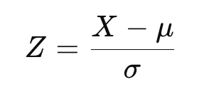
where X is the transformed data, μ is the mean, and σ is the standard deviation.

Now, if you are familiar with the distinction between population Z-score and sample Z-score, as we cover in our Statistical Inference in R track, you might recognize the above equation as the equation for a population Z-score. If you are working with a sample instead of the entire population, we would estimate the mean and standard deviation instead:

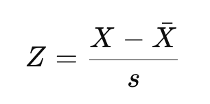
Here, X-bar is the sample mean, and s is the sample standard deviation.

The result would be the same if you used the mean and standard deviation from the new, normalized dataset. But sometimes researchers might be interested in comparing the data relative to a larger reference population by using some kind of benchmark mean and standard deviation instead.

Imagine looking at an income dataset, which would be right-skewed, and doing a log transform to normalize it. Then, imagine also that we want to compare the incomes relative to national benchmarks, in which case we would use the national mean and standard deviation instead of those from our sample to calculate Z-scores. The purpose here would be to allow for meaningful comparison across datasets or studies.

So, basically, if you're using a sample, you technically get a standardized normal approximation rather than the exact theoretical standard normal distribution. I think it's a distinction worth clarifying even if the difference must be small for large datasets.

Visualizing the Standard Normal Distribution

Here is one way to create a theoretical standard normal distribution in the R programming language. In this code, I have also added vertical lines for standard scores, AKA Z-scores, which is a way of telling us, for any given value, how many standard deviations above or below the population mean our value is. 

install.packages("ggplot2")
library(ggplot2)

ggplot(data.frame(x = c(-4, 4)), aes(x)) +
	stat_function(fun = dnorm, geom = "area", fill = '#ffe6b7', color = 'black', alpha = 0.5,  args = list( mean = 0, sd = 1)) +
	labs(title = "Standard Normal Distribution", subtitle = "Standard Deviations and Z-Scores") +
	theme(plot.title = element_text(hjust = 0.5, face = "bold")) +
	theme(plot.subtitle = element_text(hjust = 0.5)) +
	geom_vline(xintercept = 1, linetype = 'dotdash', color = "black") +
	geom_vline(xintercept = -1, linetype = 'dotdash', color = "black") +
	geom_vline(xintercept = 2, linetype = 'dotdash', color = "black") +
	geom_vline(xintercept = -2, linetype = 'dotdash', color = "black") +
	geom_vline(xintercept = 3, linetype = 'dotdash', color = "black") +
	geom_vline(xintercept = -3, linetype = 'dotdash', color = "black") +
	geom_text(aes(x=1, label="\n 1 σ", y=0.125), colour="#376795", angle=90, text=element_text(size=11)) +
	geom_text(aes(x=2, label="\n 2 σ", y=0.125), colour="#376795", angle=90, text=element_text(size=11)) +
	geom_text(aes(x=3, label="\n 3 σ", y=0.125), colour="#376795", angle=90, text=element_text(size=11)) +
	geom_text(aes(x=-1, label="\n-1 σ", y=0.125), colour="#376795", angle=90, text=element_text(size=11)) +
	geom_text(aes(x=-2, label="\n-2 σ", y=0.125), colour="#376795", angle=90, text=element_text(size=11)) +
	geom_text(aes(x=-3, label="\n-3 σ", y=0.125), colour="#376795", angle=90, text=element_text(size=11))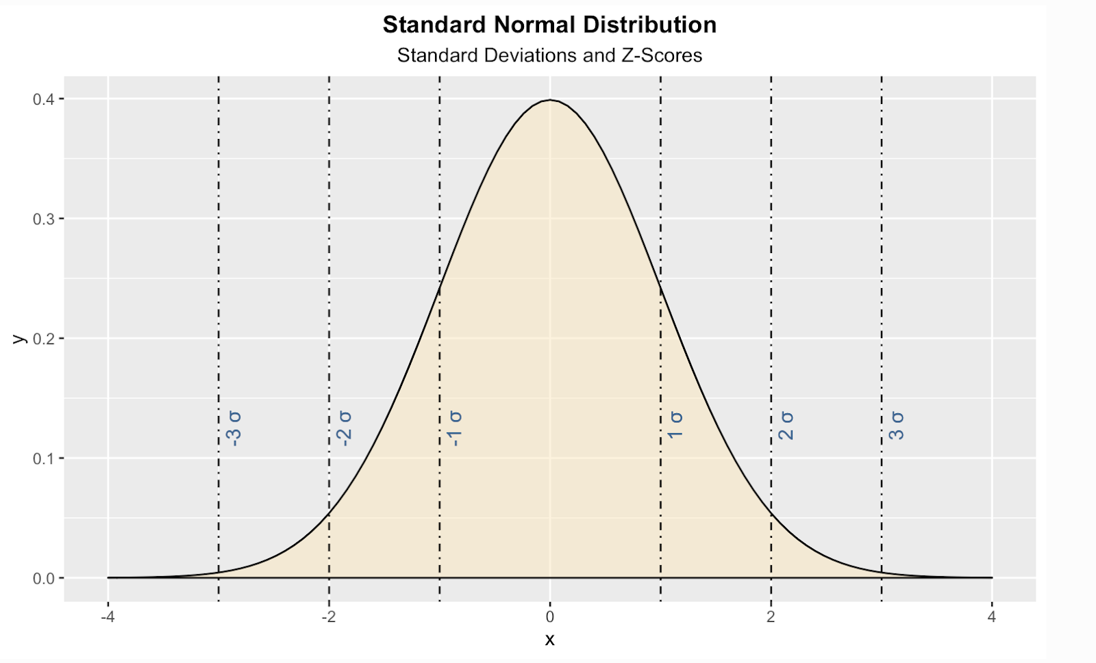

You should know there are some similar distributions that can look like standard normal but aren't:

The Standard Normal Distribution and the Standard Normal Table

Now let me go back to something I mentioned earlier: the idea of a standard normal table, also called a Z-score table, or Z-table, which is used to find cumulative probabilities for a Z-score, which represents the number of standard deviations a value is from the mean in a standard normal distribution. This table is commonly used in statistics for hypothesis testing, confidence intervals, and probability calculations. The idea here is that, instead of calculating probabilities manually, you can refer to the table to quickly determine the proportion of values that fall below a given Z-score.

The table takes a bit of practice to read, and the tables sometimes look different from each other. Here, you see it structured in a two-dimensional format. The purpose is to make it easier to look up probabilities for Z-scores when working with decimal places. In this case, the leftmost column contains the whole number and the first decimal place of the Z-score. The top row represents the second decimal place. To find the probability associated with a specific Z-score, locate the row corresponding to the first part of the Z-score, then find the column that matches the second decimal place. The value at the intersection of this row and column is the cumulative probability, meaning the proportion of data points that fall below that Z-score.

It's best to show an example: For example, suppose you calculate a Z-score of 0.32 for a student's test score. This means the score is 0.32 standard deviations above the mean. Now, let’s use the Z-table to find the probability that a randomly selected value is less than this Z-score.

• Step 1: Locate the row for 0.3.
• Step 2: Locate the column for 0.02.
• Step 3: Look at the intersection of the row for 0.3 and the column for 0.02. The value at this position is 0.6915.

The cumulative probability for Z = 0.32 is 0.6554, meaning 65.54% of values in a standard normal distribution are less than 0.32 standard deviations above the mean. If you need to determine the probability of a value being greater than a given Z-score, subtract the table value from 1 before finding the row and column.

Conclusion

I hope you enjoyed this exploration into the standard normal distribution. Keep learning with us here at DataCamp. I've mentioned our Introduction to Statistics in R course and our Statistical Inference in R skill track. But if you prefer Python, our Statistical Thinking in Python course and our Experimental Design in Python course are both great options.