Você já executou um teste t, obteve um p-valor limpo e depois percebeu que nunca verificou se seus dados tinham uma distribuição normal?

Testes estatísticos não avisam quando suas premissas são violadas. Eles apenas retornam o valor. O problema é que testes como o teste t e a ANOVA pressupõem que seus dados seguem uma distribuição normal. Se esse não for o caso, você está construindo conclusões sobre bases instáveis.

Os testes de normalidade oferecem uma maneira de verificar essa premissa. Existem métodos visuais e estatísticos para fazer isso, e saber qual usar — e como ler os resultados — é o que permite que você defenda seus resultados com confiança.

Neste artigo, vou guiá-lo pelos métodos visuais e estatísticos mais comuns para verificar a normalidade, mostrar como executá-los em Python e R e explicar o que fazer quando seus dados não passam no teste.

O que é Distribuição Normal na Prática

Você provavelmente já viu a curva de sino antes — mas aqui está o que ela realmente significa para seus dados.

Uma distribuição normal é um padrão onde a maioria dos valores se agrupa em torno do centro, e menos valores aparecem à medida que você se afasta em qualquer direção. Ao plotá-la, você obtém uma curva simétrica em forma de sino. O lado esquerdo espelha o lado direito.

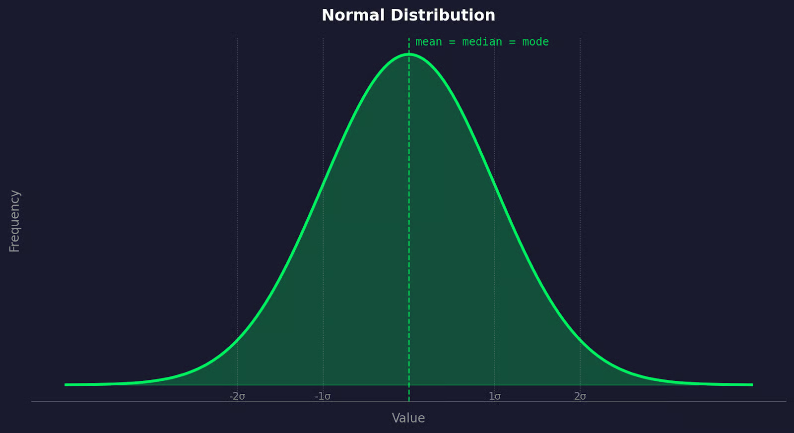
Gráfico de distribuição normal

O que torna a distribuição normal única é que a média, a mediana e a moda caem no mesmo ponto — o centro do sino. Não há assimetria para a esquerda ou para a direita. Em outras palavras, os dados são equilibrados.

Isso aparece constantemente em dados de medição do mundo real. Altura humana, leituras de pressão arterial, tolerâncias de fabricação, pontuações de testes — tudo isso tende a seguir uma distribuição normal quando você coleta amostras suficientes. A variação natural em sistemas biológicos e físicos tende a produzir esse formato.

Dito isso, nem todos os dados se comportam dessa maneira. Dados de renda são assimétricos à direita. Tempos de resposta de sites têm caudas longas.

No mundo real, as coisas podem dar muito errado se você assumir a normalidade sem verificar.

Por que Testar a Normalidade é Importante

O problema de não verificar a normalidade é que a maioria dos testes estatísticos comuns — testes t, ANOVA — são testes paramétricos.

Isso significa que eles são construídos sobre premissas sobre a distribuição dos seus dados. A normalidade é uma delas. Quando essa premissa é quebrada, a matemática do teste é quebrada junto. Você ainda obterá o resultado do teste, mas ele pode levá-lo a conclusões erradas.

Testes paramétricos funcionam fazendo suposições matemáticas sobre a população da qual sua amostra provém. Quando essas suposições se mantêm, esses testes são úteis e precisos. Quando não se mantêm, seus p-valores tornam-se não confiáveis e você não pode tirar conclusões precisas.

É aí que entram os testes não paramétricos.

Testes como Mann-Whitney U ou Kruskal-Wallis não pressupõem normalidade — eles trabalham com postos (ranks) em vez de valores brutos. Eles são mais flexíveis, mas também tendem a ser menos úteis quando seus dados são normais. Portanto, mudar para eles desnecessariamente não é a resposta.

O verdadeiro problema que tantos iniciantes em ciência de dados cometem é pular completamente a verificação.

O teste de normalidade leva algumas linhas de código. Não testar significa que você está confiando cegamente nos seus dados — ou não pensando neles de forma alguma.

Métodos Visuais para Verificar a Normalidade

Antes de executar qualquer teste formal, plote seus dados. Os visuais dirão muito sobre com o que você está trabalhando.

Histograma

Um histograma mostra o formato da sua distribuição.

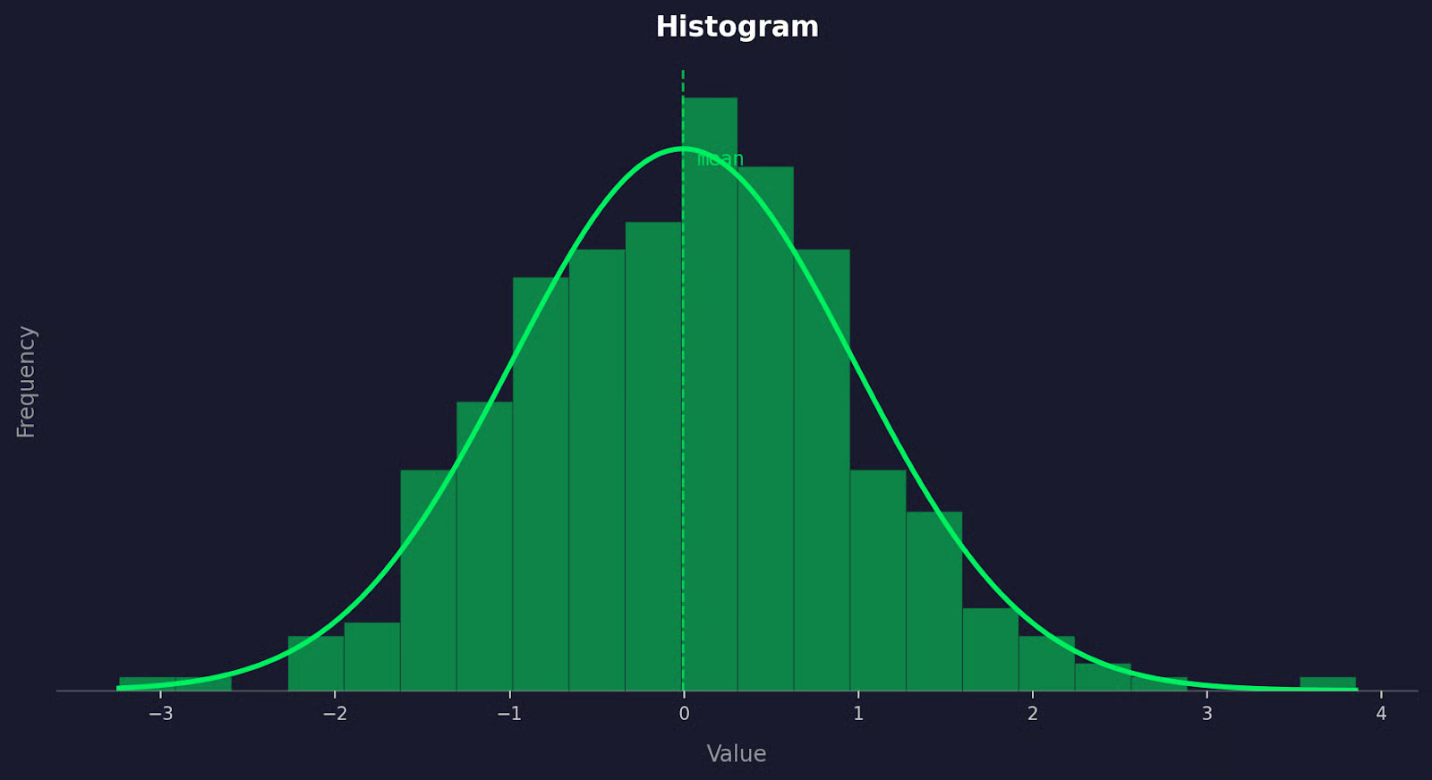
Exemplo de histograma

Se seus dados estiverem normalmente distribuídos, o histograma deve parecer uma curva de sino — alto no meio, diminuindo simetricamente em ambos os lados. O que você está observando é a assimetria (skewness): uma cauda longa puxando para a direita significa assimetria positiva, uma cauda puxando para a esquerda significa assimetria negativa. De qualquer forma, isso é um sinal de que seus dados podem não ser normais.

O problema com os histogramas é que seu formato depende do tamanho das caixas (bins):

• Poucas caixas e a distribuição parece plana
• Muitas e parece irregular

Sempre tente alguns tamanhos de caixa antes de tirar conclusões.

Gráfico Q-Q

Um gráfico Q-Q (gráfico quantil-quantil) compara os quantis dos seus dados com os quantis de uma distribuição normal teórica.

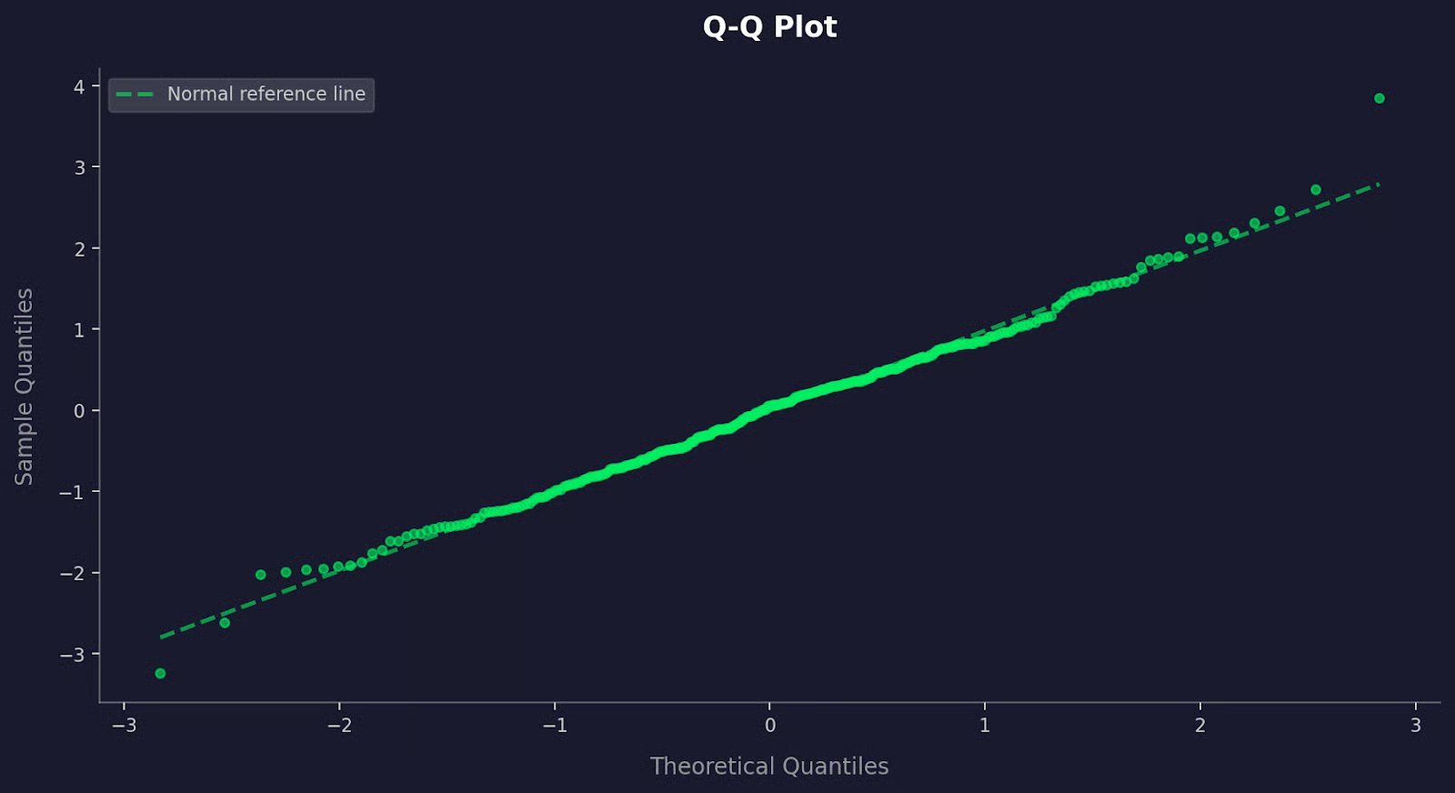
Exemplo de gráfico Q-Q

Se seus dados forem normais, os pontos caem ao longo de uma linha diagonal reta. Desvios dessa linha dizem onde a normalidade se quebra. Pontos curvando-se para cima nas extremidades sugerem caudas pesadas. Uma curva em forma de S aponta para assimetria.

Os gráficos Q-Q são mais precisos que os histogramas para detectar desvios sutis da normalidade — especialmente nas caudas, onde os histogramas tendem a perder coisas.

Box plot

Um box plot mostra a mediana, a dispersão e os outliers em uma única visualização.

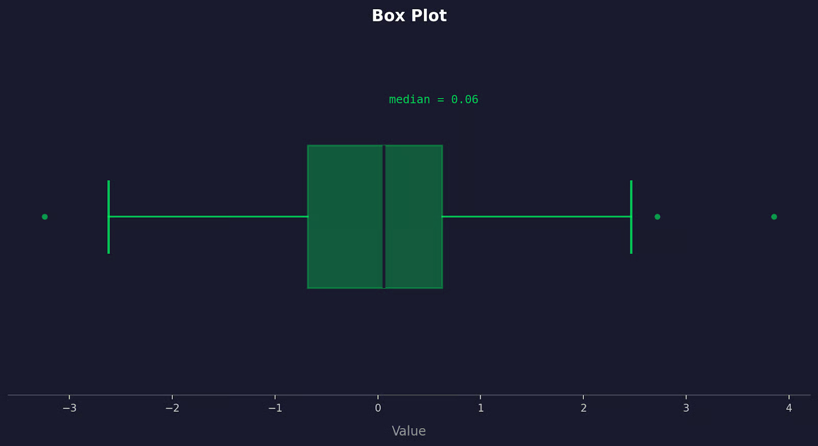
Exemplo de box plot

Um conjunto de dados normalmente distribuído produz um box plot onde a mediana fica aproximadamente no centro da caixa, e os bigodes (whiskers) se estendem por comprimentos aproximadamente iguais em ambos os lados. Se a mediana estiver fora do centro, ou um bigode for muito mais longo que o outro, isso é assimetria. Pontos fora dos bigodes são outliers.

O problema geral com os visuais é que eles são subjetivos. Duas pessoas podem olhar para o mesmo histograma e discordar. Use-os para ter uma noção dos seus dados primeiro, depois confirme com um teste formal.

Testes de Normalidade Comuns na Estatística

Não existe um único teste de normalidade que funcione melhor em todas as situações. O correto depende do tamanho da sua amostra e do que você está tentando detectar.

Teste de Shapiro-Wilk

O teste de Shapiro-Wilk é a escolha preferencial para amostras pequenas a médias, geralmente até algumas centenas de observações.

Ele mede o quão próximo seus dados correspondem a uma distribuição normal comparando os valores observados com o que você esperaria se os dados fossem normais. É amplamente utilizado, bem compreendido e disponível em todas as principais bibliotecas de estatística. Para a maioria dos analistas, este é o primeiro teste a ser considerado.

Sua principal limitação é que ele se torna excessivamente sensível com amostras grandes. Ele tende a sinalizar desvios minúsculos e praticamente sem sentido como estatisticamente significativos.

Teste de Kolmogorov-Smirnov

O teste de Kolmogorov-Smirnov (KS) compara a distribuição cumulativa da sua amostra com uma teórica — neste caso, a normal.

Ele é mais geral que o Shapiro-Wilk e pode testar contra qualquer distribuição, não apenas a normal. O teste KS é menos poderoso que o Shapiro-Wilk para testes de normalidade, o que significa que é menos provável que detecte desvios sutis. Ele também exige que você especifique os parâmetros da distribuição antecipadamente, o que introduz viés se você os estimar a partir dos mesmos dados.

Use-o quando precisar de uma verificação rápida e de uso geral — não como seu teste de normalidade principal.

Teste de Anderson-Darling

O teste de Anderson-Darling é uma variação do teste KS, mas com uma diferença fundamental: ele dá mais peso às caudas da distribuição.

Isso o torna melhor para detectar desvios que aparecem nos extremos — caudas pesadas, outliers ou comportamento não normal que o teste KS perderia. Se o seu caso de uso for sensível ao comportamento das caudas, o Anderson-Darling é uma boa escolha.

Teste de D'Agostino-Pearson

O teste de D'Agostino-Pearson adota uma abordagem diferente.

Em vez de comparar distribuições diretamente, ele mede duas propriedades dos seus dados: assimetria (skewness) e curtose (o quão pesadas ou leves são as caudas).

Ele combina ambos em uma única estatística de teste. Isso o torna bom para identificar por que seus dados podem não ser normais — não apenas se eles são. Funciona melhor com amostras maiores, onde as estimativas de assimetria e curtose são confiáveis.

Teste de Jarque-Bera

O teste de Jarque-Bera também usa assimetria e curtose, semelhante ao D'Agostino-Pearson.

É comum em econometria e análise de séries temporais. Como o D'Agostino-Pearson, ele precisa de uma amostra razoavelmente grande para produzir resultados confiáveis. Com amostras pequenas, o teste não é muito confiável. Se você estiver trabalhando em um contexto de finanças ou economia, provavelmente verá este com frequência.

Para concluir, comece com Shapiro-Wilk para amostras pequenas e combine-o com um gráfico Q-Q. Use Anderson-Darling quando o comportamento da cauda for importante e D'Agostino-Pearson quando quiser entender a natureza do desvio.

Como Interpretar os Resultados do Teste de Normalidade

Todo teste de normalidade é um teste de hipótese.

A hipótese nula em qualquer teste de normalidade é que seus dados estão normalmente distribuídos. O teste então pergunta: dado o que vemos nos dados, quão provável é que essa hipótese nula seja verdadeira?

A resposta vem como um p-valor:

• p > 0,05 — você não tem evidências suficientes para rejeitar a normalidade. Assuma que os dados são normais e prossiga com testes paramétricos
• p < 0,05 — os dados diferem da normalidade o suficiente para serem estatisticamente detectáveis. Rejeite a premissa de normalidade

Parece simples, mas muitas pessoas erram aqui.

Um p-valor baixo não diz o quão não normal seus dados são — apenas que uma diferença foi detectada. Com amostras grandes, os testes de normalidade tornam-se extremamente sensíveis. Eles sinalizarão desvios tão pequenos que não têm impacto real na sua análise.

O problema oposto também existe. Com amostras pequenas, até dados visivelmente assimétricos podem produzir p > 0,05 porque o teste não tem poder suficiente para detectar o desvio.

Significância estatística e significância prática não são a mesma coisa.

Um p-valor diz se existe um desvio da normalidade. Ele não diz se esse desvio importa para sua análise específica. Sempre combine o resultado do seu teste com um gráfico Q-Q — se os pontos seguirem a linha de perto, seus dados provavelmente são normais o suficiente, independentemente do que o p-valor diga.

Testes de Normalidade em Python

O módulo scipy.stats do Python tem tudo o que você precisa para executar testes de normalidade em algumas linhas de código.

Para todos os exemplos abaixo, usarei o mesmo conjunto de dados — 100 amostras extraídas de uma distribuição normal — para que você possa executar o código e acompanhar.

import numpy as np
from scipy import stats

np.random.seed(42)
data = np.random.normal(loc=0, scale=1, size=100)

Teste de Shapiro-Wilk

Use shapiro() como sua primeira verificação, especialmente com conjuntos de dados menores.

stat, p_value = stats.shapiro(data)
print(f"Statistic: {stat:.4f}, p-value: {p_value:.4f}")

Isso é o que você obtém:

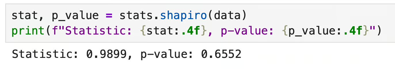
Resultado de um teste de Shapiro-Wilk em Python

O p-valor está bem acima de 0,05, então não rejeitamos a normalidade. Os dados parecem normais — o que faz sentido, já que os geramos a partir de uma distribuição normal.

Teste de Kolmogorov-Smirnov

kstest() compara sua amostra com uma distribuição nomeada. Para normalidade, passe "norm" junto com a média e o desvio padrão da amostra.

stat, p_value = stats.kstest(data, 'norm', args=(data.mean(), data.std()))
print(f"Statistic: {stat:.4f}, p-value: {p_value:.4f}")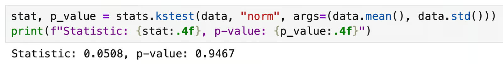

Resultado de um teste de Kolmogorov-Smirnov em Python

Novamente, p > 0,05 — nenhuma evidência contra a normalidade.

Com este teste em Python, sempre passe a média e o desvio padrão explicitamente via args. Se você pular isso, kstest() assume como padrão uma normal padrão (média=0, std=1), o que lhe dará resultados não confiáveis, a menos que seus dados já estejam padronizados.

Teste de D'Agostino-Pearson

normaltest() testa a normalidade verificando a assimetria e a curtose combinadas. Funciona melhor com amostras maiores.

stat, p_value = stats.normaltest(data)
print(f"Statistic: {stat:.4f}, p-value: {p_value:.4f}")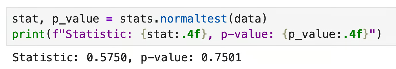

Resultado de um teste de D'Agostino-Pearson em Python

p > 0,05 novamente. Os dados passam em todos os três testes aqui, mas isso é esperado — eu os gerei para serem normais. Na prática, você frequentemente verá esses testes discordarem, especialmente perto do limite de 0,05. Quando isso acontecer, recorra ao seu gráfico Q-Q para tomar a decisão.

Testes de Normalidade em R

O R possui funções integradas para testes de normalidade. Não são necessários pacotes extras para o básico.

Assim como nos exemplos em Python, usarei o mesmo conjunto de dados: 100 amostras de uma distribuição normal.

set.seed(42)
data <- rnorm(100, mean = 0, sd = 1)

Teste de Shapiro-Wilk

shapiro.test() é a escolha certa para amostras pequenas a médias. Basta passar seu vetor de dados:

shapiro.test(data)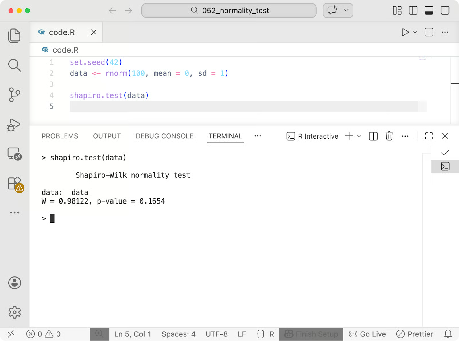

Resultado de um teste de Shapiro-Wilk em R

p > 0,05 — nenhuma evidência contra a normalidade. A estatística W varia de 0 a 1, onde valores próximos a 1 indicam que os dados seguem de perto uma distribuição normal.

Teste de Kolmogorov-Smirnov

ks.test() compara sua amostra com uma distribuição teórica. Para normalidade, especifique "pnorm" e passe a média e o desvio padrão da amostra.

ks.test(data, "pnorm", mean(data), sd(data))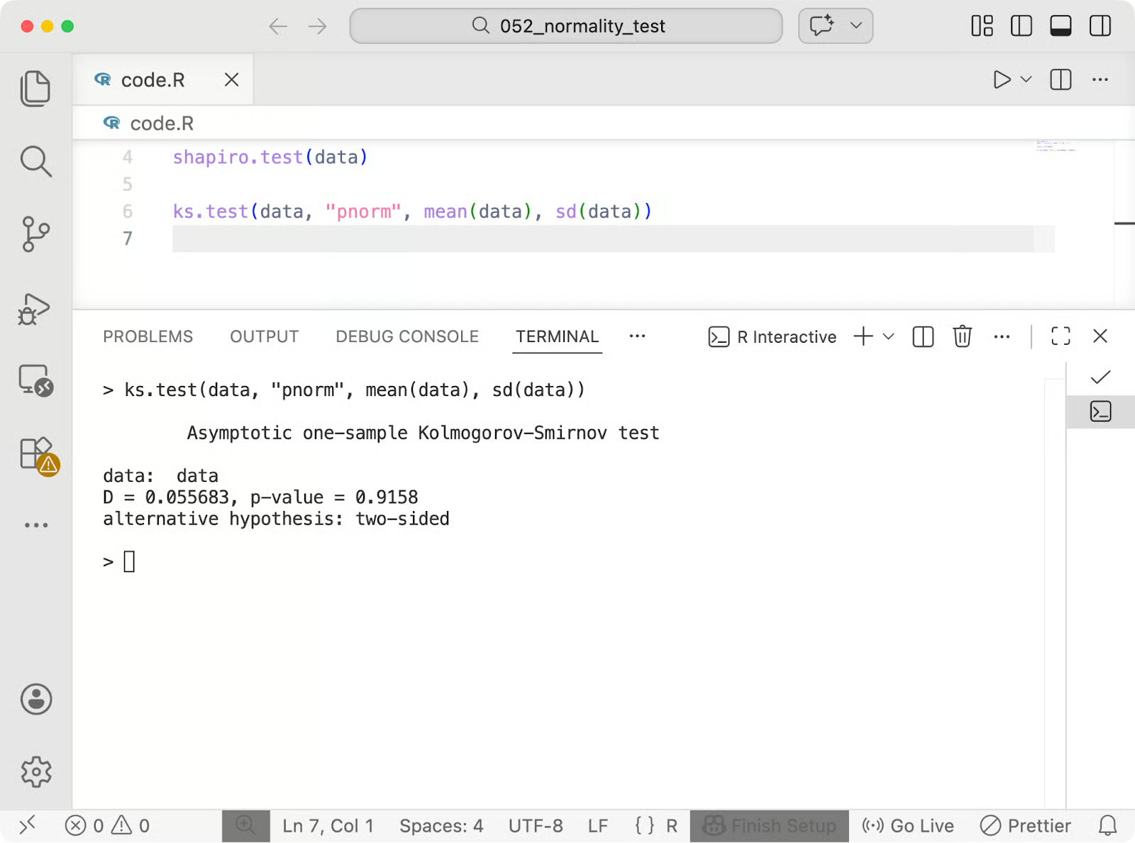

Resultado de um teste de Kolmogorov-Smirnov em R

p > 0,05 novamente. Este teste no R tem a mesma ressalva que no Python: sempre passe mean(data) e sd(data). Pular isso assumiria como padrão uma normal padrão, o que distorce o resultado, a menos que seus dados já estejam padronizados.

Gráfico Q-Q

As funções integradas do R qqnorm() e qqline() fornecem um gráfico Q-Q em duas linhas de código.

qqnorm(data, main = "Q-Q Plot")
qqline(data, col = "steelblue", lwd = 2)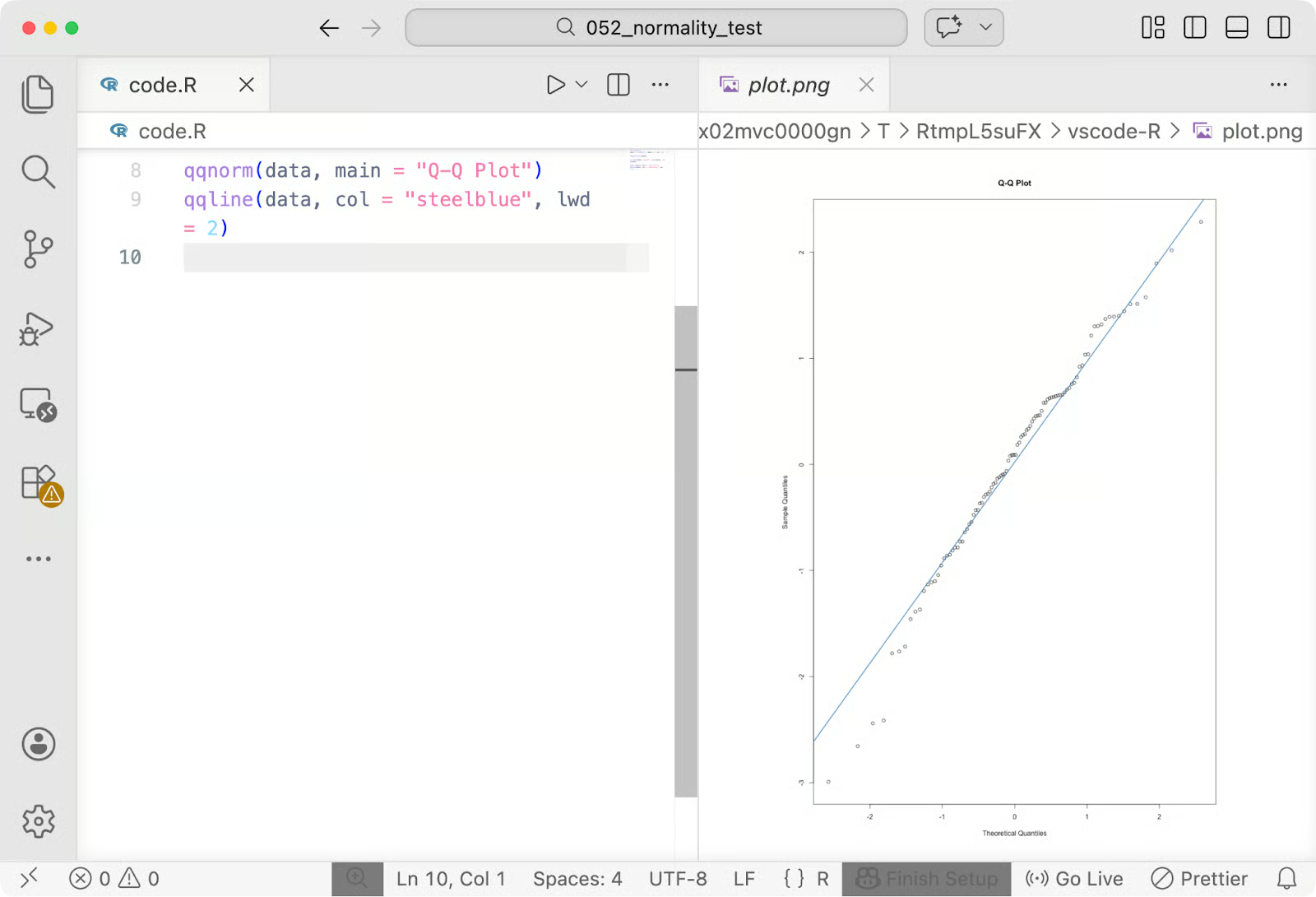

Gráfico Q-Q em R

qqnorm() plota os quantis da sua amostra contra os quantis normais teóricos. qqline() desenha a linha de referência. Pontos que seguem essa linha de perto significam que seus dados estão se comportando normalmente. Desvios nas extremidades sinalizam problemas nas caudas que valem a pena investigar.

O que Fazer se os Dados Não Forem Normais

Se seus dados falharem em um teste de normalidade, você tem algumas opções sólidas.

Transformar os dados

Às vezes, a solução é transformar seus dados para que se comportem normalmente e, em seguida, executar seus testes originais nos valores transformados.

Transformação logarítmica é a escolha mais comum. Funciona bem em dados assimétricos à direita — pense em renda, tempos de resposta ou medições biológicas que têm uma cauda longa no lado direito. A função em Python é np.log(data), e o equivalente em R é log(data).

Transformação de raiz quadrada é uma opção mais suave para assimetria moderada, e é útil quando seus dados contêm zeros (já que você não pode calcular o log de zero). Use np.sqrt(data) em Python ou sqrt(data) em R.

Após transformar, execute novamente seu teste de normalidade. Se os dados transformados passarem, prossiga com seus testes paramétricos — apenas lembre-se de interpretar os resultados em termos da escala transformada.

Usar testes não paramétricos

Se a transformação não funcionar ou não fizer sentido para seus dados, mude para testes não paramétricos. Eles não pressupõem normalidade — eles classificam os dados em vez de trabalhar com valores brutos.

• Teste de Mann-Whitney U é a alternativa não paramétrica ao teste t de amostras independentes. Use-o quando estiver comparando dois grupos
• Teste de Kruskal-Wallis é a versão não paramétrica da ANOVA de uma via. Use-o quando estiver comparando três ou mais grupos

Ambos estão disponíveis em scipy.stats (mannwhitneyu() e kruskal()) e no pacote base do R (wilcox.test() e kruskal.test()).

Confiar em amostras grandes

Com amostras grandes o suficiente, você geralmente pode ignorar a preocupação com a normalidade.

O teorema central do limite diz que, à medida que o tamanho da sua amostra cresce, a distribuição amostral da média se aproxima da normal — independentemente de como os dados originais são distribuídos. Na prática, isso significa que os testes paramétricos tendem a ser confiáveis com amostras grandes, mesmo quando os dados subjacentes não são perfeitamente normais.

Erros Comuns ao Testar a Normalidade

O teste de normalidade é fácil — você viu que leva apenas uma linha de código. Ainda assim, existem algumas maneiras de errar.

Aqui estão alguns erros comuns que iniciantes em ciência de dados costumam cometer:

• Confiar apenas em p-valores: Um p-valor diz se um desvio da normalidade foi detectado, não quão grande é esse desvio ou se ele importa. Tratar p > 0,05 como luz verde e p < 0,05 como luz vermelha é muito simplista. Sempre combine o resultado do seu teste com um gráfico Q-Q
• Ignorar os efeitos do tamanho da amostra: Com amostras pequenas, os testes de normalidade podem perder desvios reais e retornar p > 0,05 mesmo quando seus dados são visivelmente assimétricos. Com amostras grandes, o teste torna-se tão sensível que sinaliza desvios minúsculos e sem sentido como estatisticamente significativos. O tamanho da amostra pode mudar o que o p-valor significa
• Testar excessivamente a normalidade: Nem toda análise precisa de um teste formal de normalidade. Se você está fazendo um trabalho exploratório, um histograma e um gráfico Q-Q geralmente são suficientes
• Interpretar mal pequenos desvios: Dados do mundo real quase nunca são perfeitamente normais. Um pequeno desvio da linha de referência em um gráfico Q-Q, ou um p-valor logo abaixo de 0,05, não significa que seus dados estão longe da normalidade. A questão é se eles são normais o suficiente para o teste que você está executando

Portanto, para concluir, o teste de normalidade é apenas uma verificação dos seus dados. Use-o como uma entrada entre muitas, não como a palavra final.

Quando Você Pode Pular o Teste de Normalidade

O teste de normalidade nem sempre é necessário. Se você estiver com um prazo apertado, saber quando pular pode economizar tempo sem afetar os resultados.

Grandes conjuntos de dados

Quando você tem uma amostra grande, o teorema central do limite garante que a distribuição amostral da média seja aproximadamente normal, independentemente do formato dos seus dados brutos. Os testes paramétricos são geralmente confiáveis nessa situação, então executar um teste formal de normalidade agrega pouco valor.

Alguns métodos estatísticos também são robustos à não normalidade. Técnicas como regressão linear tendem a se manter bem quando os tamanhos das amostras são razoáveis e as violações não são extremas. (A regressão linear ainda pressupõe normalidade nos resíduos.)

Análise exploratória

Quando você está examinando dados em busca de padrões, construindo intuição ou decidindo quais variáveis investigar mais a fundo, um histograma ou gráfico Q-Q rápido é suficiente. Testes formais são para análise confirmatória — quando suas conclusões precisam se sustentar.

Lembre-se de que o teste de normalidade existe para protegê-lo de tirar conclusões erradas. Se você está em um contexto onde uma conclusão errada não traz consequências reais, ou onde seu método não depende da normalidade, o teste é opcional.

Conclusão

O teste de normalidade serve para verificar se suas premissas se mantêm bem o suficiente para confiar nos seus resultados.

Nenhum conjunto de dados é perfeitamente normal. O objetivo é entender como seus dados se comportam e escolher seus métodos de acordo. Um gráfico Q-Q diz onde estão os desvios. Um teste formal informa se eles são estatisticamente detectáveis. Quando combinados, eles dão uma imagem mais clara do que qualquer um deles sozinho.

O teste certo depende do seu contexto. Use Shapiro-Wilk para amostras pequenas, Anderson-Darling quando as caudas importam, alternativas não paramétricas quando a normalidade não pode ser assumida. E, às vezes — com amostras grandes ou métodos robustos — nenhum teste.

Você acha o conceito de p-valores confuso? Leia nosso artigo Teste de Hipótese Facilitado para garantir que você os está interpretando corretamente.