Programa
Gradient descent is one of the most important algorithms in all of machine learning and deep learning. It is an extremely powerful optimization algorithm that can train linear regression, logistic regression, and neural network models. If you are getting into machine learning, it is therefore imperative to understand the gradient descent algorithm in-depth.
What is Gradient Descent?
Data science is about discovering complex patterns and behaviors in big data analysis. These are called "patterns," i.e., recurring motifs. Through machine learning, this is a matter of training algorithms to detect patterns in data analysis to perform a specific task better. This means teaching software to perform a task or make predictions autonomously. To do this, the data scientist selects and trains algorithms to perform data analysis. The goal is, of course, to improve their predictions over time.
Consequently, machine learning is largely based on the training of algorithms. The more these algorithms are exposed to data, the more they learn to perform a task without specific instructions; they learn by experience. We use different types of algorithms in machine learning. Among them, gradient descent is one of the most useful and popular.
Gradient descent is an optimization algorithm. It is used to find the minimum value of a function more quickly. The definition of gradient descent is rather simple. It is an algorithm to find the minimum of a convex function. To do this, it iteratively changes the parameters of the function in question. It is an algorithm that is used, for example, in linear regression.
A convex function is a function that looks like a beautiful valley with a global minimum in the center. Conversely, a non-convex function is a function that has several local minima, and the gradient descent algorithm should not be used on these functions at the risk of getting stuck at the first minima encountered.
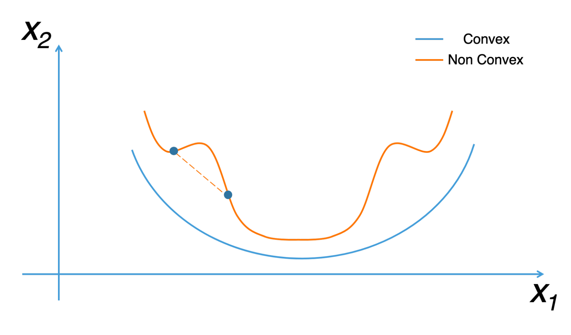
Gradient descent is also called “the deepest downward slope algorithm”. It is very important in machine learning, where it is used to minimize a cost function. The latter is used to determine the best prediction model in data analysis. The more the cost is minimized, the more the machine will be able to make good predictions.
You will find three well-known types of descent. Let's take a closer look at them:
Batch gradient descent
Also known as vanilla gradient descent, batch gradient descent calculates the errors for each example in the training dataset. However, it does so only after each training example has been rigorously evaluated. It is fair to compare this process to a cycle. Some people also refer to it as a training era.
Batch descent has several advantages. In particular, its computational efficiency is extremely practical because it develops stable convergence and a stable error gradient. That said, batch gradient descent also has some drawbacks. Sometimes, its stable error gradient can lead to an unfavorable convergence state. In addition, it also needs the presence of the training data set in its algorithm and memory.
Stochastic gradient descent
Stochastic gradient descent provides individual parameter updates for each training example. It allows attention to be paid to each example, ensuring that the process is error-free. Depending on the problem, this can help the SGD become faster compared to batch gradient descent. Its regular updates provide us with detailed improvement rates.
That said, these updates are computationally expensive, especially when compared to the approach used by stepwise descent. In addition, the frequency of updates can cause noisy gradients and could prevent the error rate from decreasing. Instead, the error rate jumps and becomes problematic in the long run.
Mini-batch gradient descent
Scientists use mini-batch gradient descent as a starting method. Why? Because it is a perfect blend of the concepts of stochastic descent and batch descent. It divides data sets (training) into batches and performs an update for each batch, creating a balance between the efficiency of BGD and the robustness of DDC.
Popular mini-batches range from fifty, to two hundred and fifty-six, but like many other machine learning methods, there are no clear rules as it varies from application to application. People use it as a basic option for training neural networks. It is also a popular type of hill descent in the deep learning landscape.
Why is Gradient Descent so Important in Machine Learning?
In machine learning, we use the gradient descent algorithm in supervised learning problems to minimize the cost function, which is a convex function (for example, the mean square error).
Thanks to this algorithm, the machine learns by finding the best model. Remember that minimizing the cost function means finding the parameters a, b, c, etc., that give the smallest errors between our model and the y points of the dataset. Once the cost function is minimized, this opens the door to building accurate voice recognition programs, computer vision programs, and applications to predict the stock market price.
You can see why the gradient descent algorithm is fundamental: the machine learns from it.
To better illustrate the functioning and usefulness of this algorithm, we often use the analogy of the mountain. We imagine a person who has lost his way in the mountains. Basically, it will be a matter of finding the way back by first looking for the direction with a steep downward slope. After having followed this direction for a certain distance, this method must be repeated until a valley is reached (the lowest value). In machine learning, the gradient descent consists of repeating this method in a loop until finding a minimum for the cost function. This is why it is called an iterative algorithm and why it requires a lot of calculation.
Here is a 2-step strategy that will help you out if you are lost in the mountains:
- From your current position, you look all around you for the direction of where the slope is going down the hardest.
- Once you find that direction, you follow it for a distance (say you walk 300 meters) and repeat step 1.
By repeating steps 1 and 2 in a loop, you are sure to converge on the minimum of the valley. This strategy is nothing more or less than the gradient descent algorithm.
Step 1: Compute the derivative of the cost function
We start from a random initial point and then measure the value of the slope at that point. In mathematics, you measure a slope by calculating the derivative of the function.
Step 2: Updating the model parameters
We then progress by a certain distance d in the slope direction, which goes down, but not 300 meters this time. This distance is called the “learning rate.” The result of this operation is to modify the value of the parameters of our model (our coordinates in the valley change when we move).
Which Fields Use Gradient Descent?
The gradient descent algorithm is mostly used in the fields of machine learning and deep learning. The latter can be considered as an improved version of machine learning. It allows for the detection of the most subtle patterns. These are disciplines that require a strong background in mathematics and a background in Python.
This programming language has several libraries that facilitate the application of machine learning. This discipline is very useful for analyzing large volumes of data accurately and quickly. It allows predictive analysis based on past trends or events.
Machine learning is one of the sciences that are closely related to big data in terms of opportunities to exploit. It allows overcoming the limits of human intelligence in the analysis of large data streams. With the vast data sets available online, artificial intelligence (AI) can learn on its own without human intervention. Machine learning is used, for example, in the field of connected objects. Thanks to it, an AI can adapt to the habits of the occupants of a connected house and execute its tasks taking these habits into account.
For example, AI can adjust the heating of a room according to the weather. It is this science that also allows us to have more and more sophisticated robot vacuum cleaners. Gradient descent through machine learning is at the heart of the great advances in artificial intelligence. In practice, there are many applications of gradient descent by engineers and AI specialists.
It is useful for search engines like Google, and popular recommendation engines like YouTube, Netflix, or Amazon. Based on the data collected from users, the algorithms will try to understand the interests of the internet user. This will allow them to offer relevant search results and better recommendations.
Machine learning has enabled computers to understand and process human language. It is this application that gave birth to digital assistants like Alexa, Google Assistant, and Siri. Machine learning and applications of gradient descent are also very useful for video game developers. Here the goal is to enable AIs to excel at the most human tasks in order to enable people to focus on high-value activities. Artificial intelligence and machine learning allow companies to anticipate their customers' needs and future trends.
How to Implement Gradient Descent
Gradient descent is an algorithm used in linear regression because of the computational complexity. The general mathematical formula for gradient descent is xt+1= xt- η∆xt, with η representing the learning rate and ∆xt the direction of descent. Gradient descent is an algorithm applicable to convex functions. Taking ƒ as a convex function to be minimized, the goal will be to obtain ƒ(xt+1) ≤ ƒ (xt) at each iteration.
The idea here is to use this algorithm which will gradually compute the minimum of a mathematical function. When faced with certain equations, this is the best way to solve them. When we talk about gradient descent, we must also understand the notion of a cost function. In a supervised mode, this function allows measuring the margin of error between an estimate and the real value. The formula to compute the mean square gradient in the case of a linear regression problem is the following:
The application of gradient descent also uses the notion of learning rate. It is a hyperparameter that allows control of the adjustment of the network weights with respect to the loss gradient. It should be noted that an optimal learning rate is very important to obtain a minimum more quickly and efficiently. It should be neither too high nor too low.
As the value goes down, it shows that one is gradually moving along the downward slope. Several optimization methods use the gradient descent algorithm, such as RMSprop, Adam, and SGD. In order not to make mistakes when using this algorithm, it is recommended to choose its parameters carefully. One should also keep in mind that the minimum found might not be considered as a global minimum.
The primary function of a gradient is to measure the change in each weight against the change in the errors. Think of gradients as the slope of a function. The slope will be steeper the higher the gradient - this is a favorable condition for models because they can learn quickly. However, the model will stop learning if the slope becomes zero. Mathematically speaking, a gradient could be described as a finite derivative with respect to its inputs.
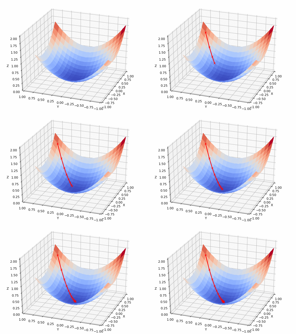
In the implementation part, we will write two functions. One will be the cost function which takes the actual output and predicted output as input and returns the loss. The second one will be the actual gradient descent function which takes the independent variable and the target variable(dependent variable) as input and finds the best fitting line using the gradient descent algorithm.
The iterations, learning rate, and stopping threshold are the tuning parameters of the gradient descent algorithm and can be set by the user. In the main function, we will initialize random linearly related data, and apply the gradient descent algorithm on the data to find the best fitting line. The optimal weight and bias found using the gradient descent algorithm are then used to draw the line of best fit in the main function.
#Importing libraries
import numpy as np
import matplotlib as pyplot

def mean_squared_error(y_true, y_predicted):

   # Calculating the loss or cost
   cost = np.sum((y_true-y_predicted)**2) / len(y_true)
   return cost

# Gradient descent function
# Here iterations, learning rate, stopping threshold are hyperparameters that can be tuned
def gradient_descent((x, y, iterations = 1000, learning_rate = 0.0001, stopping_theshold = 1e-6):

   #Initialzing rate, bias, learning rate, and iterations
   current_rate = 0.1
   current_bias = 0.01
   iterations = iterations
   learning_rate = learning_rate
   n = float(len(x))

   costs = []
   weights = []
   previous_cost = None

   # Estimation of optimal parameters
   for i in range(iterations):

      # Making predictions
      y_predicted = (current_weight * x) + current_bias

      # Calculating the current cost
      current_cost = mean_squared_error(y, y_predicted)

      # If the change in cost is less than or equal to stopping threshold we stop the gradient descent
      if previous_cost and abs(previous_cost - current_cost) <= stopping_threshold:
         break

      previous_cost = current_cost

      costs.append(current_cost)
      weights.append(current_weight)

      # Calculating the gradients
      weight_derivative = -(2/n) * sum(x * (y-y_predicted))
      bias_derivative = -(2/n) * sum(y-y_predicted)

      # Updating weights and bias
      current_weight = current_weight - (learning_rate * weight_derivative)
      current_bias = current_bias - (learning_rate * bias_derivative)

      # Printing the parameters for each 1000th iteration
      print(f"Iteration {i+1}: Cost {current_cost}, Weight \n {current_weight}, Bias {current_bias}")

   # Visualizing the weights and cost for all iterations
   plt.figure(figsize = = (8,6))
   plt.plot(weights, cost)
   plt.scatter(weights, cost, marker = 'o', color = 'red')
   plt.title("Cost vs Weights")
   plt.ylabel("Cost")
   plt.xlabel("Weights")
   plt.show()

   return current_weight, current_bias

def main()

   # Data
   X = np.array(32.5, 53.4, 61.5, 47.4, 59.8,
   55.1, 52.2, 39.2, 48.1, 52.5,
   45.4, 54.3, 44.1, 58.1, 56.7,
   48.9, 44.6, 60.2, 45.6, 38.8])
   Y = np.array(31.7, 68.7, 62.5, 71.5, 87.2,
   78.2, 79.6, 59.1, 75.3, 71.3,
   55.1, 82.4, 62.0, 75.3, 81.4,
   60.7, 82.8, 97.3, 48.8, 56.8])

   # Estimating weight and bias using gradient descent
   estimated_weight, estimated_bias = gradient_descent(X, Y, iterations = 2000)
   print(f"Estimated Weight: {estimated weight}\nEstimated Bias: {estimated bias}")

   # Making predictions using estimated parameters
   Y_pred = estimated_weight*X = estimated_bias

   #Plotting the regression line
   plt.figure(figsize = 8,6)
   plt.scatter(X, Y, marker = 'o', color = 'red')
   plt.plot([min(X), max(X)], [min(Y_pred), max(Y_pred)], color = 'blue')
   plt.ylabel("X")
   plt.xlabel("Y")
   plt.show()

if __name__=="__main__":
   main()
The output of the code below will be as follows:
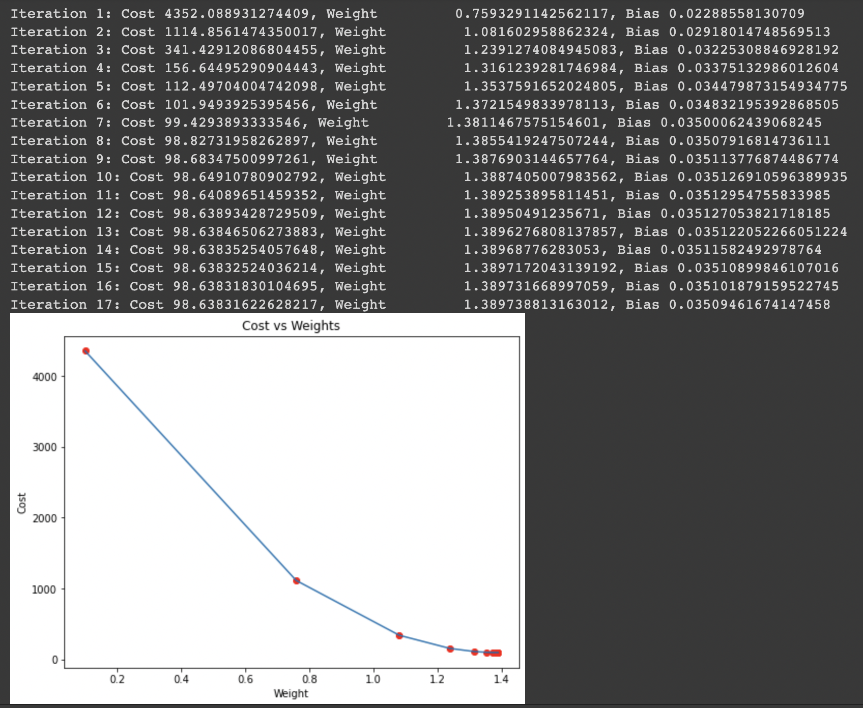
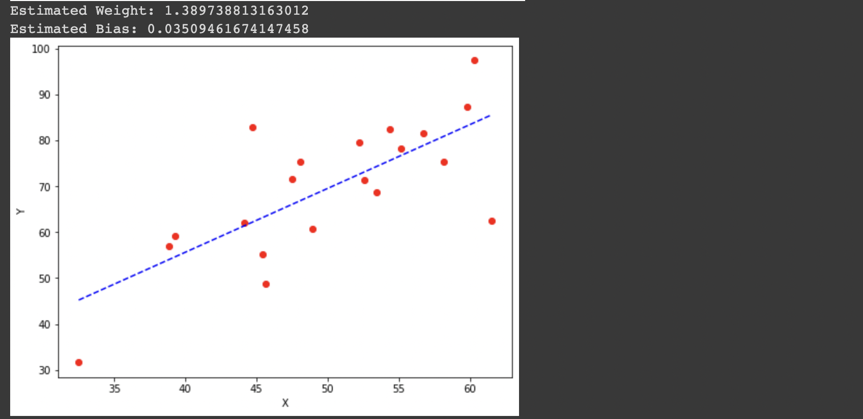
You can test and run the code above with this notebook.
Learning Rate: the Role of the Hyper-parameter
Another element that is important to emphasize is the learning rate. In machine learning, we call this kind of factor a hyper-parameter because it is not strictly speaking a parameter of our model, but it still has an impact on the final performance of our model (just like the model parameters).
The learning rate (often noted α or sometimes η) indicates the speed at which the coefficients evolve. This quantity can be fixed or variable. One of the most popular methods at the moment is called Adam, which has a learning rate that scales over time.
There are many scenarios to expect and to take into consideration while using gradient descent :
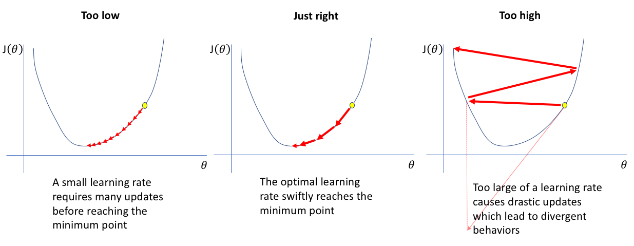
Learning rate too high
If the learning rate is too big, then you will make too big steps in the gradient descent. This has the advantage of going down quickly to the minimum of the cost function, but you risk missing this minimum by oscillating around it at infinity. In the valley analogy, it's as if you were moving several kilometers each time, thus passing the shelter without realizing it.
Learning rate too small
To avoid the previous case, you might be tempted to choose a very low learning rate. But if it is too small, then you risk taking an infinite amount of time before converging to the minimum of the cost function. It's a bit like choosing to go millimeter by millimeter up the mountain to find the lowest point in the valley.
- Why are learning rates so important?
It is essential to set learning rates to appropriate values to help the descent of slopes reach local minimums. Therefore, it would be best not to set them too high or too low. This is essential because reaching the minimum could become complicated with too-long steps. Therefore, if we set the learning rates to lower values, the gradient descent might eventually reach its local minima. However, this may take some time.
- How to find the best learning rates
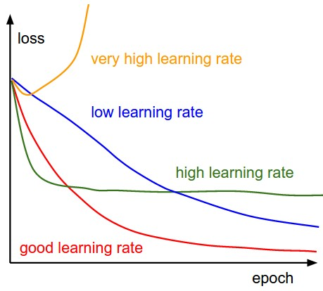
Unfortunately, there is no magic formula to find the right learning rate. Most of the time, you have to fumble around and try several values before you find the right one. This is called hyperparameter tuning, and there are different strategies to do this properly.
A great way to ensure optimal operation of the slope descent is to arrange the cost function while the optimization is in progress. Enter the number of repetitions on the X-axis, and the value of the cost function will enter on the Y-axis. This will help you see the value of the cost function after each gradient descent iteration while allowing you to track the accuracy of the learning rate. You can also try different values and plot them together.
The cost function will decrease after each iteration if the gradient descent is working optimally. Gradient descent converges when it fails to reduce the cost function, and stays at the same level. The number of iterations required for gradient descent to converge varies considerably. Sometimes it takes fifty iterations, and other times it can be as many as two or three million. It is difficult to estimate the number of iterations in advance.
Some algorithms can tell you automatically if there has been a convergence in the gradient descent. However, it would be better to establish a convergence threshold in advance, which is also quite difficult to estimate. This is an important reason why simple plots are best for convergence tests.
Conclusion
While scientists use gradient descent to find the values of a function's parameters to minimize function costs, programmers use gradient descent as an optimization algorithm when training machine learning models. Gradient descent iteratively adjusts some of its parameters to minimize a particular function based on convex functions.
Gradient descent is probably the most recognized optimization strategy used in deep learning and machine learning. Data scientists often use it when there is a chance to combine each algorithm with learning models. Understanding the gradient descent algorithm is relatively simple, and implementing it is even simpler. To dive deeper into the realm of deep learning, check out our full catalog of machine learning courses.
Become an ML Scientist
Gradient Descent FAQs
What is gradient descent?
Gradient descent is an optimization algorithm used to minimize the cost function in machine learning and deep learning models. It iteratively updates model parameters in the direction of the steepest descent to find the lowest point (minimum) of the function.
How does gradient descent work?
Gradient descent works by calculating the gradient (or slope) of the cost function with respect to each parameter. Then, it adjusts the parameters in the opposite direction of the gradient by a step size, or learning rate, to reduce the error.
What is the learning rate in gradient descent?
The learning rate is a hyperparameter that controls the size of the steps taken toward the minimum of the cost function. A smaller learning rate results in slower convergence, while a larger learning rate may cause the algorithm to overshoot the minimum.
What are the common challenges of gradient descent?
Gradient descent can face challenges such as getting stuck in local minima, slow convergence, and sensitivity to the choice of learning rate. Techniques like momentum, adaptive learning rates (Adam, RMSprop), and regularization can help address these issues.


