What is Normalization in Machine Learning? A Comprehensive Guide to Data Rescaling

In machine learning, the foundation for successful models is built on the quality of data they are trained on. While the spotlight often shines on complex, sophisticated algorithms and models, the unsung hero is often data preprocessing. Data preprocessing is an important step that transforms raw data into features that is then used for effective machine learning.

Machine learning algorithms are often trained with the assumption that all features contribute equally to the final prediction. However, this assumption fails when the features differ in range and unit, hence affecting their importance.

Enter normalization – a vital step in data preprocessing that ensures uniformity of the numerical magnitudes of features. This uniformity avoids the domination of features that have larger values compared to the other features or variables.

In this article, we will dive into normalization, a feature scaling technique that offers a pathway to balance the scales of the features.

What is Normalization?

Normalization is a specific form of feature scaling that transforms the range of features to a standard scale. Normalization and, for that matter, any data scaling technique is required only when your dataset has features of varying ranges. Normalization encompasses diverse techniques tailored to different data distributions and model requirements.

Normalization is not limited to just numeric data. However, in this article, we will focus on numeric examples. Be sure to check out Datacamp’s Textacy: An introduction to text data cleaning and normalization in Python tutorial if you are planning to perform preprocessing on text data for machine learning.

Why Normalize Data?

Normalized data enhances model performance and improves the accuracy of a model. It aids algorithms that rely on distance metrics, such as k-nearest neighbors or support vector machines, by preventing features with larger scales from dominating the learning process.

Normalization fosters stability in the optimization process, promoting faster convergence during gradient-based training. It mitigates issues related to vanishing or exploding gradients, allowing models to reach optimal solutions more efficiently.

Normalized data is also easy to interpret and thus, easier to understand. When all the features of a dataset are on the same scale, it also becomes easier to identify and visualize the relationships between different features and make meaningful comparisons.

Let’s take a simple example to highlight the importance of normalizing data. We are trying to predict housing prices based on various features such as square footage, number of bedrooms, and distance to the supermarket, etc. The dataset contains diverse features with varying scales, such as:

• Square footage: Ranges from 500 to 5000 square feet
• Number of bedrooms: Ranges from 1 to 5
• Distance to supermarket: Ranges from 0.1 to 10 miles

When you feed this data without any preprocessing directly to a machine learning model, the algorithm might give more weight to features with large scales, such as square footage. During training, the algorithm assumes that a change in total square footage will have a significant impact on housing prices. The algorithm might overlook the nuances of features that are relatively small, such as the number of bedrooms and distance to the supermarket. This skewed emphasis can lead to suboptimal model performance and biased predictions.

By normalizing the features, we can ensure that each feature contributes proportionally to the model's learning process. The model can now learn patterns across all features more effectively, leading to a more accurate representation of the underlying relationships in the data.

Normalization Techniques at a Glance

Min-Max scaling and Z-score normalization (standardization) are the two fundamental techniques for normalization. Apart from these, we will also discuss decimal scaling normalization, log scaling normalization, and robust scaling, which address unique challenges in data preprocessing.

Min-Max Scaling

Min-max scaling is very often simply called ‘normalization.’ It transforms features to a specified range, typically between 0 and 1. The formula for min-max scaling is:

X_normalized = X – X_min / X_max – X_min

Where X is a random feature value that is to be normalized. X_min is the minimum feature value in the dataset, and X_max is the maximum feature value.

• When X is minimum value, the numerator is zero (X_min - X_min) and hence, the normalized value is 0
• When X is maximum value, the numerator is equal to the denominator (X_max - X_min) and hence, the normalized value is 1
• When X is neither minimum or maximum, the normalized value is between 0 and 1. This is referred to as min-max scaling technique

Min-max scaling is a good choice when:

• The approximate upper and lower bounds of the dataset is known, and the dataset has few or no outliers
• When the data distribution is unknown or non-Gaussian, and the data is approximately uniformly distributed across the range
• When maintaining the distribution’s original shape is essential

Z-score normalization (standardization)

Z-score normalization (standardization) assumes a Gaussian (bell curve) distribution of the data and transforms features to have a mean (μ) of 0 and a standard deviation (σ) of 1. The formula for standardization is:

X_standardized = X−μ / σ

​This technique is particularly useful when dealing with algorithms that assume normally distributed data, such as many linear models. Unlike the min-max scaling technique, feature values are not restricted to a specific range in the standardization technique. This normalization technique basically represents features in terms of the number of standard deviations that lie away from the mean.

Before we delve into other data transformation techniques, let’s perform a comparison of normalization (min-max scaling) and standardization.

Decimal scaling normalization

The objective of decimal scaling normalization is to scale the feature values by a power of 10, ensuring that the largest absolute value in each feature becomes less than 1. It is useful when the range of values in a dataset is known, but the range varies across features. The formula for decimal scaling normalization is:

X_decimal = X / 10^d

Where X is the original feature value, and d is the smallest integer such that the largest absolute value in the feature becomes less than 1.

For example, if the largest absolute value in a feature is 3500, then d would be 3, and the feature would be scaled by 10³.

Decimal scaling normalization is advantageous when dealing with datasets where the absolute magnitude of values matters more than their specific scale.

Log scaling normalization

Log scaling normalization converts data into a logarithmic scale, by taking the log of each data point. It is particularly useful when dealing with data that spans several orders of magnitude. The formula for log scaling normalization is:

X_log = log(X)

This normalization comes in handy with data that follows an exponential growth or decay pattern. It compresses the scale of the dataset, making it easier for models to capture patterns and relationships in the data. Population size over the years is a good example of a dataset where some features exhibit exponential growth. Log scaling normalization can make these features more amenable to modeling.

Robust scaling normalization

Robust scaling normalization is useful when working with datasets that have outliers. It uses the median and interquartile range (IQR) instead of the mean and standard deviation to handle outliers. The formula for robust scaling is:

X_robust = X – median/ IQR

Since robust scaling is resilient to the influence of outliers, this makes it suitable for datasets with skewed or anomalous values.

Common Normalization Pitfalls and Best Practices

We have discussed normalization and why it’s useful in machine learning. Although powerful, normalization is not without its challenges. From handling outliers to selecting the most appropriate technique based on your dataset, addressing these issues is essential to unleash the full potential of your machine learning model.

Handling outliers

Outliers are data points in your dataset that significantly deviate from the norm and distort the effectiveness of normalization techniques. If you do not handle outliers in your data, these can lead to skewed transformations. You can work with the robust scaling normalization technique we discussed earlier to handle outliers.

Another strategy is to apply trimming or winsorizing, where we identify and either clip or cap all feature values above (or below) a certain value to fixed value.

Choice of normalization technique

We have discussed the most useful normalization techniques, but there are many more to choose from. Selecting the appropriate technique requires a nuanced understanding of the dataset. When data preprocessing, you need to try multiple normalization techniques and assess their impact on model performance. Experimentation allows you to observe how each method influences the learning process.

You need to gain a deep understanding of the data’s characteristics. Consider whether the assumptions of a specific normalization technique align with the distribution and patterns present in the dataset.

Normalization on sparse data

Normalization can be challenging when dealing with sparse data where many feature values are zero. Applying standard normalization techniques directly may lead to unintended consequences. There are versions of the normalization techniques we discussed above that are specifically designed for sparse data, such as ‘sparse min-max scaling.’

Before normalization, consider imputing or handling missing values in your dataset. This is often one of the first steps when you are exploring your dataset and cleaning it for usage in machine learning models.

Make sure to check out DataCamp’s Feature Engineering for Machine Learning course, which gives you hands-on experience on how to prepare any data for your own machine learning models. In the course, you will work with Stack Overflow Developers survey, and historic US presidential inauguration addresses to understand how best to preprocess and engineer features from categorical, continuous, and unstructured data.

Normalization and the risk of overfitting

In machine learning, overfitting occurs when a model learns not only the underlying patterns in the training data but also captures noise and random fluctuations. This can lead to a model that performs exceptionally well on the training data but fails to generalize to new, unseen data.

Normalization alone may not cause overfitting. However, when normalization is combined with other factors, such as the complexity of the model or insufficient regularization, it can contribute to overfitting. When normalization parameters are calculated using the entire dataset (including validation or test sets), it can lead to data leakage. The model might inadvertently learn information from the validation or test sets, compromising its ability to generalize.

Thus, to mitigate the risk of overfitting, normalize the training set and apply the same normalization parameters to the validation and test sets. This ensures that the model learns to generalize from the training data without being influenced by information in the validation or test sets.

You need to implement proper regularization techniques to penalize overly complex models. Regularization helps prevent the model from fitting noise in the training data. Use proper validation techniques, such as cross-validation, to assess the model's performance on unseen data. If overfitting is detected during validation, adjustments can be made, such as reducing model complexity or increasing regularization.

Implementing Normalization in Python with Scikit-learn

Scikit-learn is a versatile Python library that is engineered to simplify the intricacies of machine learning. It provides a rich set of tools and functionalities for data preprocessing, feature selection, dimensionality reduction, building and training models, model evaluation, hyperparameter tuning, model serialization, pipeline construction, etc. Its modular design encourages experimentation and exploration, allowing users to seamlessly transition from fundamental concepts to advanced methodologies.

We will use scikit-learn to put what we learned into practice. We will use the classic and widely used `Iris dataset.` This dataset was introduced by the British biologist and statistician Ronald A. Fisher in 1936. The Iris dataset comprises measurements of four features from three different species of iris flowers: setosa, versicolor, and virginica.

There are four features measured for each flower, these are the sepal length, sepal width, petal length, and petal width - all in centimeters. There are 150 instances (samples) in the dataset, with 50 samples from each of the three species. The Iris dataset is usually used for classification tasks, where the goal is to predict the correct species among the three classes. However, today, we will use this dataset to show the transformation of the data when applying normalization (min-max scaling) and standardization. 

You can execute the below-discussed Python code in Datacamp’s workspace to explore the dataset yourself.

Let’s start with importing the libraries we need….

import numpy as np
import pandas as pd
# To import the dataset
from sklearn.datasets import load_iris
# To be used for splitting the dataset into training and test sets
from sklearn.model_selection import train_test_split
# To be used for min-max normalization
from sklearn.preprocessing import MinMaxScaler
# To be used for Z-normalization (standardization)
from sklearn.preprocessing import StandardScaler

# Load the iris dataset from Scikit-learn package
iris = load_iris()

# This prints a summary of the characteristics, statistics of the dataset
print(iris.DESCR)
 
# Divide the data into features (X) and target (Y)
# Data is converted to a panda’s dataframe
X = pd.DataFrame(iris.data)
 
# Separate the target attribute from rest of the data columns
Y = iris.target
 
# Take a look at the dataframe
X.head()
 
# This prints the shape of the dataframe (150 rows and 4 columns)
X.shape()

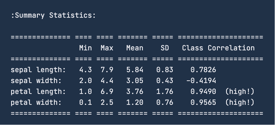
When you check out the summary statistics for the data using print(iris.DESCR), the image below is the summary you will receive. For the feature ‘sepal length’, the range is 4.3 – 7.9 centimeters. Similarly, for ‘sepal width’, the range is 2 – 4.4 centimeters. For ‘petal length’ the range is 1-6.9 centimeters and finally, for ‘petal width’ the range is 0.1 – 2.5 centimeters.

Before we apply normalization, it is a good practice to divide the dataset into training and test sets. We will use train_test_split functionality from sklearn.model_selection to do so. We are not carving out a validation set since we will not be performing actual machine learning modeling in this exercise. We will make an 80-20 split of the dataset, which means the training set will have 120 rows, and the test will have the rest 30 data points.

# To divide the dataset into training and test sets

X_train, X_test, y_train, y_test = train_test_split(X, Y ,test_size=0.2)

A usual step after loading the data and dividing the data into a training-testing set is to perform data cleaning, data imputing to handle missing values and to handle data outliers. However, since the focus of the article is on normalization – we will skip these preprocessing steps and jump to see normalization in action.

We will now transform this data to fall under the range of 0 – 1 centimeter using min-max normalization technique. To normalize the data, we will use the MinMaxScaler functionality from sklearn library and apply it to our dataset; we have already imported the required libraries earlier.

# Good practice to keep original dataframes untouched for reusability
X_train_n = X_train.copy()
X_test_n = X_test.copy()
 
# Fit min-max scaler on training data
norm = MinMaxScaler().fit(X_train_n)
 
# Transform the training data
X_train_norm = norm.transform(X_train_n)
 
# Use the same scaler to transform the testing set
X_test_norm = norm.transform(X_test_n)

We can print the training data to see the transformation that occurred. However, let's convert the set into a pandas dataframe and then check its statistical description using the describe() functionality.

X_train_norm_df = pd.DataFrame(X_train_norm)
 
     	# Assigning original feature names for ease of read
X_train_norm_df.columns = iris.feature_names
 
X_train_norm_df.describe()

This will give the following result for normalization:

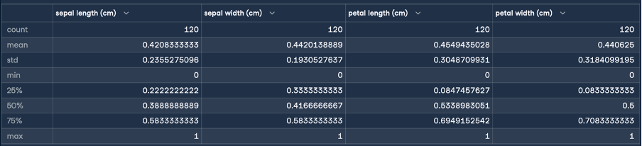
Here, the min and max statistics indicate that the ranges of the features have all been transformed to a range of 0 – 1 centimeter. This is the transformation we were aiming for! We will now perform standardization (Z-score normalization) by following the same steps as we did for normalization:

X_train_s = X_train.copy()
X_test_s = X_test.copy()
 
# Fit the standardization scaler onto the training data
stan = StandardScaler().fit(X_train_s)
 
# Transform the training data
X_train_stan = stan.transform(X_train_s)
 
# Use the same scaler to transform the testing set
X_test_stan = stan.transform(X_test_s)
 
     	# Convert the transformed data into pandas dataframe
X_train_stan_df = pd.DataFrame(X_train_stan)
 
     	# Assigning original feature names for ease of read
X_train_stan_df.columns = iris.feature_names
 
     	# Check out the statistical description
X_train_stan_df.describe()

This will give the following result for standardization:

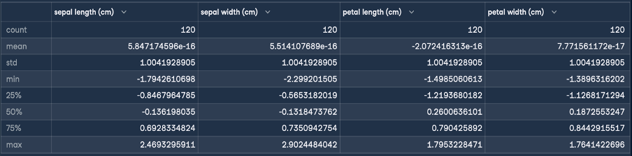
The objective of Z-normalization is to transform the values of a feature to have a mean of 0 and a standard deviation of 1. As you can see from the dataframe’s description that was generated, the mean for all four features is a small number close to zero, and the standard deviation is 1.

We can now take this transformed data and feed it to a machine learning algorithm for training.

Final Thoughts

In this article, we've journeyed through min-max scaling, Z-normalization, decimal scaling, and log scaling normalizations. Each technique revealed its unique strengths and usefulness. You’ve also read about some of the common pitfalls and best practices when performing normalization. Finally, we wrapped up by applying some of this newly acquired knowledge to use, with scikit learn.

To learn more about the concepts and processes we’ve covered, check out our courses on Feature Engineering for Machine Learning in Python and Textacy: An Introduction to Text Data Cleaning and Normalization in Python.