HomeTutorialsMachine Learning

Support Vector Machines with Scikit-learn Tutorial

In this tutorial, you'll learn about Support Vector Machines, one of the most popular and widely used supervised machine learning algorithms.
Updated Dec 2019  · 15 min read

SVM offers very high accuracy compared to other classifiers such as logistic regression, and decision trees. It is known for its kernel trick to handle nonlinear input spaces. It is used in a variety of applications such as face detection, intrusion detection, classification of emails, news articles and web pages, classification of genes, and handwriting recognition.

In this tutorial, you will be using scikit-learn in Python. If you would like to learn more about this Python package, I recommend you take a look at our Supervised Learning with scikit-learn course.

SVM is an exciting algorithm and the concepts are relatively simple. The classifier separates data points using a hyperplane with the largest amount of margin. That's why an SVM classifier is also known as a discriminative classifier. SVM finds an optimal hyperplane which helps in classifying new data points.

In this tutorial, you are going to cover following topics:

Watch and learn more about Support Vector Machines with Scikit-learn in this video from our course.

Support Vector Machines

Generally, Support Vector Machines is considered to be a classification approach, it but can be employed in both types of classification and regression problems. It can easily handle multiple continuous and categorical variables. SVM constructs a hyperplane in multidimensional space to separate different classes. SVM generates optimal hyperplane in an iterative manner, which is used to minimize an error. The core idea of SVM is to find a maximum marginal hyperplane(MMH) that best divides the dataset into classes.

Support Vectors

Support Vectors

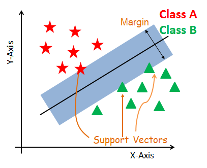
Support vectors are the data points, which are closest to the hyperplane. These points will define the separating line better by calculating margins. These points are more relevant to the construction of the classifier.

Hyperplane

A hyperplane is a decision plane which separates between a set of objects having different class memberships.

Margin

A margin is a gap between the two lines on the closest class points. This is calculated as the perpendicular distance from the line to support vectors or closest points. If the margin is larger in between the classes, then it is considered a good margin, a smaller margin is a bad margin.

How does SVM work?

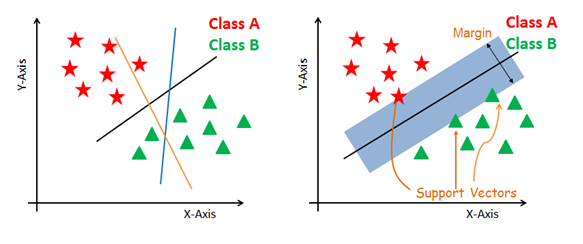
The main objective is to segregate the given dataset in the best possible way. The distance between the either nearest points is known as the margin. The objective is to select a hyperplane with the maximum possible margin between support vectors in the given dataset. SVM searches for the maximum marginal hyperplane in the following steps:

  1. Generate hyperplanes which segregates the classes in the best way. Left-hand side figure showing three hyperplanes black, blue and orange. Here, the blue and orange have higher classification error, but the black is separating the two classes correctly.

  2. Select the right hyperplane with the maximum segregation from the either nearest data points as shown in the right-hand side figure.

Linear Separator

Dealing with non-linear and inseparable planes

Some problems can’t be solved using linear hyperplane, as shown in the figure below (left-hand side).

In such situation, SVM uses a kernel trick to transform the input space to a higher dimensional space as shown on the right. The data points are plotted on the x-axis and z-axis (Z is the squared sum of both x and y: z=x^2=y^2). Now you can easily segregate these points using linear separation.

Higher Dimension

SVM Kernels

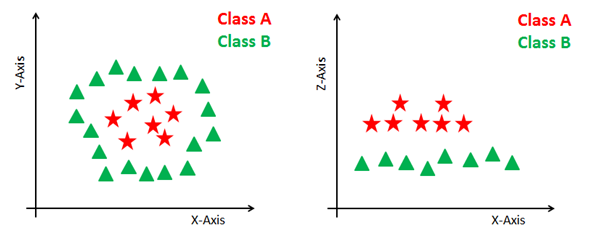
The SVM algorithm is implemented in practice using a kernel. A kernel transforms an input data space into the required form. SVM uses a technique called the kernel trick. Here, the kernel takes a low-dimensional input space and transforms it into a higher dimensional space. In other words, you can say that it converts nonseparable problem to separable problems by adding more dimension to it. It is most useful in non-linear separation problem. Kernel trick helps you to build a more accurate classifier.

  • Linear Kernel A linear kernel can be used as normal dot product any two given observations. The product between two vectors is the sum of the multiplication of each pair of input values.
K(x, xi) = sum(x * xi)
  • Polynomial Kernel A polynomial kernel is a more generalized form of the linear kernel. The polynomial kernel can distinguish curved or nonlinear input space.
K(x,xi) = 1 + sum(x * xi)^d

Where d is the degree of the polynomial. d=1 is similar to the linear transformation. The degree needs to be manually specified in the learning algorithm.

  • Radial Basis Function Kernel The Radial basis function kernel is a popular kernel function commonly used in support vector machine classification. RBF can map an input space in infinite dimensional space.
K(x,xi) = exp(-gamma * sum((x – xi^2))

Here gamma is a parameter, which ranges from 0 to 1. A higher value of gamma will perfectly fit the training dataset, which causes over-fitting. Gamma=0.1 is considered to be a good default value. The value of gamma needs to be manually specified in the learning algorithm.

Classifier Building in Scikit-learn

Until now, you have learned about the theoretical background of SVM. Now you will learn about its implementation in Python using scikit-learn.

In the model the building part, you can use the cancer dataset, which is a very famous multi-class classification problem. This dataset is computed from a digitized image of a fine needle aspirate (FNA) of a breast mass. They describe characteristics of the cell nuclei present in the image.

The dataset comprises 30 features (mean radius, mean texture, mean perimeter, mean area, mean smoothness, mean compactness, mean concavity, mean concave points, mean symmetry, mean fractal dimension, radius error, texture error, perimeter error, area error, smoothness error, compactness error, concavity error, concave points error, symmetry error, fractal dimension error, worst radius, worst texture, worst perimeter, worst area, worst smoothness, worst compactness, worst concavity, worst concave points, worst symmetry, and worst fractal dimension) and a target (type of cancer).

This data has two types of cancer classes: malignant (harmful) and benign (not harmful). Here, you can build a model to classify the type of cancer. The dataset is available in the scikit-learn library or you can also download it from the UCI Machine Learning Library.

Run and edit the code from this tutorial online

Run Code

Loading Data

Let's first load the required dataset you will use.

#Import scikit-learn dataset library
from sklearn import datasets

#Load dataset
cancer = datasets.load_breast_cancer()

Exploring Data

After you have loaded the dataset, you might want to know a little bit more about it. You can check feature and target names.

# print the names of the 13 features
print("Features: ", cancer.feature_names)

# print the label type of cancer('malignant' 'benign')
print("Labels: ", cancer.target_names)
Features:  ['mean radius' 'mean texture' 'mean perimeter' 'mean area'
 'mean smoothness' 'mean compactness' 'mean concavity'
 'mean concave points' 'mean symmetry' 'mean fractal dimension'
 'radius error' 'texture error' 'perimeter error' 'area error'
 'smoothness error' 'compactness error' 'concavity error'
 'concave points error' 'symmetry error' 'fractal dimension error'
 'worst radius' 'worst texture' 'worst perimeter' 'worst area'
 'worst smoothness' 'worst compactness' 'worst concavity'
 'worst concave points' 'worst symmetry' 'worst fractal dimension']
Labels:  ['malignant' 'benign']

Let's explore it for a bit more. You can also check the shape of the dataset using shape.

# print data(feature)shape
cancer.data.shape
(569, 30)

Let's check top 5 records of the feature set.

# print the cancer data features (top 5 records)
print(cancer.data[0:5])
[[1.799e+01 1.038e+01 1.228e+02 1.001e+03 1.184e-01 2.776e-01 3.001e-01
  1.471e-01 2.419e-01 7.871e-02 1.095e+00 9.053e-01 8.589e+00 1.534e+02
  6.399e-03 4.904e-02 5.373e-02 1.587e-02 3.003e-02 6.193e-03 2.538e+01
  1.733e+01 1.846e+02 2.019e+03 1.622e-01 6.656e-01 7.119e-01 2.654e-01
  4.601e-01 1.189e-01]
 [2.057e+01 1.777e+01 1.329e+02 1.326e+03 8.474e-02 7.864e-02 8.690e-02
  7.017e-02 1.812e-01 5.667e-02 5.435e-01 7.339e-01 3.398e+00 7.408e+01
  5.225e-03 1.308e-02 1.860e-02 1.340e-02 1.389e-02 3.532e-03 2.499e+01
  2.341e+01 1.588e+02 1.956e+03 1.238e-01 1.866e-01 2.416e-01 1.860e-01
  2.750e-01 8.902e-02]
 [1.969e+01 2.125e+01 1.300e+02 1.203e+03 1.096e-01 1.599e-01 1.974e-01
  1.279e-01 2.069e-01 5.999e-02 7.456e-01 7.869e-01 4.585e+00 9.403e+01
  6.150e-03 4.006e-02 3.832e-02 2.058e-02 2.250e-02 4.571e-03 2.357e+01
  2.553e+01 1.525e+02 1.709e+03 1.444e-01 4.245e-01 4.504e-01 2.430e-01
  3.613e-01 8.758e-02]
 [1.142e+01 2.038e+01 7.758e+01 3.861e+02 1.425e-01 2.839e-01 2.414e-01
  1.052e-01 2.597e-01 9.744e-02 4.956e-01 1.156e+00 3.445e+00 2.723e+01
  9.110e-03 7.458e-02 5.661e-02 1.867e-02 5.963e-02 9.208e-03 1.491e+01
  2.650e+01 9.887e+01 5.677e+02 2.098e-01 8.663e-01 6.869e-01 2.575e-01
  6.638e-01 1.730e-01]
 [2.029e+01 1.434e+01 1.351e+02 1.297e+03 1.003e-01 1.328e-01 1.980e-01
  1.043e-01 1.809e-01 5.883e-02 7.572e-01 7.813e-01 5.438e+00 9.444e+01
  1.149e-02 2.461e-02 5.688e-02 1.885e-02 1.756e-02 5.115e-03 2.254e+01
  1.667e+01 1.522e+02 1.575e+03 1.374e-01 2.050e-01 4.000e-01 1.625e-01
  2.364e-01 7.678e-02]]

Let's take a look at the target set.

# print the cancer labels (0:malignant, 1:benign)
print(cancer.target)
[0 0 0 0 0 0 0 0 0 0 0 0 0 0 0 0 0 0 0 1 1 1 0 0 0 0 0 0 0 0 0 0 0 0 0 0 0
 1 0 0 0 0 0 0 0 0 1 0 1 1 1 1 1 0 0 1 0 0 1 1 1 1 0 1 0 0 1 1 1 1 0 1 0 0
 1 0 1 0 0 1 1 1 0 0 1 0 0 0 1 1 1 0 1 1 0 0 1 1 1 0 0 1 1 1 1 0 1 1 0 1 1
 1 1 1 1 1 1 0 0 0 1 0 0 1 1 1 0 0 1 0 1 0 0 1 0 0 1 1 0 1 1 0 1 1 1 1 0 1
 1 1 1 1 1 1 1 1 0 1 1 1 1 0 0 1 0 1 1 0 0 1 1 0 0 1 1 1 1 0 1 1 0 0 0 1 0
 1 0 1 1 1 0 1 1 0 0 1 0 0 0 0 1 0 0 0 1 0 1 0 1 1 0 1 0 0 0 0 1 1 0 0 1 1
 1 0 1 1 1 1 1 0 0 1 1 0 1 1 0 0 1 0 1 1 1 1 0 1 1 1 1 1 0 1 0 0 0 0 0 0 0
 0 0 0 0 0 0 0 1 1 1 1 1 1 0 1 0 1 1 0 1 1 0 1 0 0 1 1 1 1 1 1 1 1 1 1 1 1
 1 0 1 1 0 1 0 1 1 1 1 1 1 1 1 1 1 1 1 1 1 0 1 1 1 0 1 0 1 1 1 1 0 0 0 1 1
 1 1 0 1 0 1 0 1 1 1 0 1 1 1 1 1 1 1 0 0 0 1 1 1 1 1 1 1 1 1 1 1 0 0 1 0 0
 0 1 0 0 1 1 1 1 1 0 1 1 1 1 1 0 1 1 1 0 1 1 0 0 1 1 1 1 1 1 0 1 1 1 1 1 1
 1 0 1 1 1 1 1 0 1 1 0 1 1 1 1 1 1 1 1 1 1 1 1 0 1 0 0 1 0 1 1 1 1 1 0 1 1
 0 1 0 1 1 0 1 0 1 1 1 1 1 1 1 1 0 0 1 1 1 1 1 1 0 1 1 1 1 1 1 1 1 1 1 0 1
 1 1 1 1 1 1 0 1 0 1 1 0 1 1 1 1 1 0 0 1 0 1 0 1 1 1 1 1 0 1 1 0 1 0 1 0 0
 1 1 1 0 1 1 1 1 1 1 1 1 1 1 1 0 1 0 0 1 1 1 1 1 1 1 1 1 1 1 1 1 1 1 1 1 1
 1 1 1 1 1 1 1 0 0 0 0 0 0 1]

Splitting Data

To understand model performance, dividing the dataset into a training set and a test set is a good strategy.

Split the dataset by using the function train_test_split(). you need to pass 3 parameters features, target, and test_set size. Additionally, you can use random_state to select records randomly.

# Import train_test_split function
from sklearn.model_selection import train_test_split

# Split dataset into training set and test set
X_train, X_test, y_train, y_test = train_test_split(cancer.data, cancer.target, test_size=0.3,random_state=109) # 70% training and 30% test

Generating Model

Let's build support vector machine model. First, import the SVM module and create support vector classifier object by passing argument kernel as the linear kernel in SVC() function.

Then, fit your model on train set using fit() and perform prediction on the test set using predict().

#Import svm model
from sklearn import svm

#Create a svm Classifier
clf = svm.SVC(kernel='linear') # Linear Kernel

#Train the model using the training sets
clf.fit(X_train, y_train)

#Predict the response for test dataset
y_pred = clf.predict(X_test)

Evaluating the Model

Let's estimate how accurately the classifier or model can predict the breast cancer of patients.

Accuracy can be computed by comparing actual test set values and predicted values.

#Import scikit-learn metrics module for accuracy calculation
from sklearn import metrics

# Model Accuracy: how often is the classifier correct?
print("Accuracy:",metrics.accuracy_score(y_test, y_pred))
Accuracy: 0.9649122807017544

Well, you got a classification rate of 96.49%, considered as very good accuracy.

For further evaluation, you can also check precision and recall of model.

# Model Precision: what percentage of positive tuples are labeled as such?
print("Precision:",metrics.precision_score(y_test, y_pred))

# Model Recall: what percentage of positive tuples are labelled as such?
print("Recall:",metrics.recall_score(y_test, y_pred))
Precision: 0.9811320754716981
Recall: 0.9629629629629629

Well, you got a precision of 98% and recall of 96%, which are considered as very good values.

Tuning Hyperparameters

  • Kernel: The main function of the kernel is to transform the given dataset input data into the required form. There are various types of functions such as linear, polynomial, and radial basis function (RBF). Polynomial and RBF are useful for non-linear hyperplane. Polynomial and RBF kernels compute the separation line in the higher dimension. In some of the applications, it is suggested to use a more complex kernel to separate the classes that are curved or nonlinear. This transformation can lead to more accurate classifiers.
  • Regularization: Regularization parameter in python's Scikit-learn C parameter used to maintain regularization. Here C is the penalty parameter, which represents misclassification or error term. The misclassification or error term tells the SVM optimization how much error is bearable. This is how you can control the trade-off between decision boundary and misclassification term. A smaller value of C creates a small-margin hyperplane and a larger value of C creates a larger-margin hyperplane.
  • Gamma: A lower value of Gamma will loosely fit the training dataset, whereas a higher value of gamma will exactly fit the training dataset, which causes over-fitting. In other words, you can say a low value of gamma considers only nearby points in calculating the separation line, while the a value of gamma considers all the data points in the calculation of the separation line.

Advantages

SVM Classifiers offer good accuracy and perform faster prediction compared to Naïve Bayes algorithm. They also use less memory because they use a subset of training points in the decision phase. SVM works well with a clear margin of separation and with high dimensional space.

Disadvantages

SVM is not suitable for large datasets because of its high training time and it also takes more time in training compared to Naïve Bayes. It works poorly with overlapping classes and is also sensitive to the type of kernel used.

Conclusion

Congratulations, you have made it to the end of this tutorial!

In this tutorial, you covered a lot of ground about Support vector machine algorithm, its working, kernels, hyperparameter tuning, model building and evaluation on breast cancer dataset using the Scikit-learn package. You have also covered its advantages and disadvantages. I hope you have learned something valuable!

To learn more about this type of classifiers, you should take a look at our Linear Classifiers in Python course. It introduces other types of regression and loss functions, as well as Support Vector Machines.

I look forward to hearing any feedback or questions. You can ask the question by leaving a comment and I will try my best to answer it.

Topics

Scikit-learn Courses

Course

Supervised Learning with scikit-learn

4 hr
110.5K
Grow your machine learning skills with scikit-learn in Python. Use real-world datasets in this interactive course and learn how to make powerful predictions!
See DetailsRight Arrow
Start Course
See MoreRight Arrow
Related

Exploring Matplotlib Inline: A Quick Tutorial

Learn how matplotlib inline can enable you to display your data visualizations directly in a notebook quickly and easily! In this article, we cover what matplotlib inline is, how to use it, and how to pair it with other libraries to create powerful visualizations.
Amberle McKee's photo

Amberle McKee

How to Use the NumPy linspace() Function

Learn how to use the NumPy linspace() function in this quick and easy tutorial.
Adel Nehme's photo

Adel Nehme

Python Absolute Value: A Quick Tutorial

Learn how to use Python's abs function to get a number's magnitude, ignoring its sign. This guide explains finding absolute values for both real and imaginary numbers, highlighting common errors.
Amberle McKee's photo

Amberle McKee

How to Check if a File Exists in Python

Learn how to check if a file exists in Python in this simple tutorial
Adel Nehme's photo

Adel Nehme

Writing Custom Context Managers in Python

Learn the advanced aspects of resource management in Python by mastering how to write custom context managers.
Bex Tuychiev's photo

Bex Tuychiev

How to Convert a List to a String in Python

Learn how to convert a list to a string in Python in this quick tutorial.
Adel Nehme's photo

Adel Nehme

See MoreSee More