Course
This tutorial will guide you on how to use TensorBoard, which is an amazing utility that allows you to visualize data and how it behaves. You will see for what sort of purposes you can use it when training a neural network.
- First, you will learn how to start TensorBoard, followed by an overview of the different views offered.
- Next, you will see how you can visualize scalar values produced during computations. You will also learn how to get insights from the model to fix any potential errors in the learning.
- Thereafter, you will investigate how you can visualize vectors or collections of data as histograms.
- With this view you will compare how weight initialization of the neural network affects the weight update of the neural network during the learning.
Tip: check out DataCamp's Deep Learning course with Keras here.
Before you get started, make sure to import the following libraries to run the code successfully:
from pandas_datareader import data
import matplotlib.pyplot as plt
import pandas as pd
import datetime as dt
import urllib.request, json
import os
import numpy as np

# This code has been tested with TensorFlow 1.6
import tensorflow as tf
from tensorflow.examples.tutorials.mnist import input_data
Starting TensorBoard
To visualize things via TensorBoard, you first need to start its service. For that,
- Open up the command prompt (Windows) or terminal (Ubuntu/Mac)
- Go into the project home directory
- If you are using Python virtuanenv, activate the virtual environment you have installed TensorFlow in
- Make sure that you can see the TensorFlow library through Python. For that,
- Type in
python3, you will get a>>>looking prompt - Try
import tensorflow as tf - If you can run this successfully you are fine
- Type in
- Exit the Python prompt (that is,
>>>) by typingexit()and type in the following commandtensorboard --logdir=summaries--logdiris the directory you will create data to visualize- Files that TensorBoard saves data into are called event files
- Type of data saved into the event files is called summary data
- Optionally you can use
--port=<port_you_like>to change the port TensorBoard runs on
- You should now get the following message
TensorBoard 1.6.0 at <url>:6006 (Press CTRL+C to quit)
- Enter the <url>:6006 in to the web browser
- You should be able to see a orange dashboard at this point. You won't have anything to display because you haven't generated data.
Note: TensorBoard does not like to see multiple event files in the same directory. This can lead to you getting very gruesome curves on the display. So you should create a separate folder for each different example (for example, summaries/first, summaries/second, ...) to save data. Another thing to keep in mind is that, if you want to re-run an experiment (that is, saving an event file to an already populated folder), you have to make sure to first delete the existing event files.
Different Views of TensorBoard
Different views take inputs of different formats and display them differently. You can change them on the orange top bar.
- Scalars - Visualize scalar values, such as classification accuracy.
- Graph - Visualize the computational graph of your model, such as the neural network model.
- Distributions - Visualize how data changes over time, such as the weights of a neural network.
- Histograms - A fancier view of the distribution that shows distributions in a 3-dimensional perspective
- Projector - Can be used to visualize word embeddings (that is, word embeddings are numerical representations of words that capture their semantic relationships)
- Image - Visualizing image data
- Audio - Visualizing audio data
- Text - Visualizing text (string) data
In this tutorial, you will cover the views shown in bold.
Understanding the Benefits of Scalar Visualization
In this section, you will first understand why visualizing certain metrics (for example loss or accuracy) is beneficial. When training deep neural networks, one of the crucial issues that strikes the beginners is the lack of understanding the effects of various design choices and hyperparameters.
For example, if you carelessly initialize weights of a deep neural network to have a very large variance between weights, your model will quickly diverge and collapse. On the other hand, things can go wrong even when you are quite competent in taming neural networks to make use of them. For example, not paying attention to the learning rate can lead to either the divergence of the model or pre-maturely saturating to sub-optimal performance.
One way to quickly detect problems with your model is to have a graphical visualization of what's going on in your model in real time (for example, every 100 iterations). So if your model is behaving oddly, it will be clearly visible. That is exactly what TensorBoard provides you with. You can decide which values need to be displayed and it will maintain a real time visualization of those values during learning.
You start by first creating a five-layer neural network that you will use to classify hand-written digit images. For that you will use the famous MNIST dataset. TensorFlow provides a simple API to load MNIST data, so you don't have to manually download it. Before that you define a simple method (that is, accuracy()), which calculates the accuracy of some predictions with respect to the true labels.
def accuracy(predictions,labels):
    '''
    Accuracy of a given set of predictions of size (N x n_classes) and
    labels of size (N x n_classes)
    '''
    return np.sum(np.argmax(predictions,axis=1)==np.argmax(labels,axis=1))*100.0/labels.shape[0]
Define Inputs, Outputs, Weights and Biases
First, define a batch_size denoting the amount of data you sample at a single optimization/validation or testing step. Then you define the layer_ids, which gives an identifier for each of the layers of the neural network you will be defining. You then can define layer_sizes.
Note that len(layer_sizes) should be len(layer_ids)+1, because layer_sizes includes the size of the input at the beginning.
MNIST has images of size 28x28, which will be 784 when unwrapped to a single dimension. Then you can define the input and label placeholders, that you will later use to train the model. Finally, you define two TensorFlow variables for each layer (that is, weights and bias).
You can use variable scoping (more information here) so that the variables will be nicely named and will be much easier to access later.
batch_size = 100
layer_ids = ['hidden1','hidden2','hidden3','hidden4','hidden5','out']
layer_sizes = [784, 500, 400, 300, 200, 100, 10]

tf.reset_default_graph()

# Inputs and Labels
train_inputs = tf.placeholder(tf.float32, shape=[batch_size, layer_sizes[0]], name='train_inputs')
train_labels = tf.placeholder(tf.float32, shape=[batch_size, layer_sizes[-1]], name='train_labels')

# Weight and Bias definitions
for idx, lid in enumerate(layer_ids):

    with tf.variable_scope(lid):
        w = tf.get_variable('weights',shape=[layer_sizes[idx], layer_sizes[idx+1]],
                            initializer=tf.truncated_normal_initializer(stddev=0.05))
        b = tf.get_variable('bias',shape= [layer_sizes[idx+1]],
                            initializer=tf.random_uniform_initializer(-0.1,0.1))
Calculating Logits, Predictions, Loss and Optimization
With the input/output placeholders, weights and biases of each layer defined, you now can define the calculations to calculate the logits of the neural network. Logits are the unnormalized values produced in the last layer of the neural network. When normalized, you call them predictions. This involves iterating through each layer in the neural network and computing tf.matmul(h,w) +b. You also need to apply an activation function like tf.nn.relu(tf.matmul(h,w) +b) for all layers except for the last one.
Next, you define the loss function that is used to optimize the neural network. In this example, you can use the cross entropy loss, which often delivers better results in classification problems than the mean squared error.
Finally, you will need to define an optimizer that takes in the loss and updates the weights of the neural network in the direction that minimizes the loss.
# Calculating Logits
h = train_inputs
for lid in layer_ids:
    with tf.variable_scope(lid,reuse=True):
        w, b = tf.get_variable('weights'), tf.get_variable('bias')
        if lid != 'out':
          h = tf.nn.relu(tf.matmul(h,w)+b,name=lid+'_output')
        else:
          h = tf.nn.xw_plus_b(h,w,b,name=lid+'_output')

tf_predictions = tf.nn.softmax(h, name='predictions')
# Calculating Loss
tf_loss = tf.reduce_mean(tf.nn.softmax_cross_entropy_with_logits_v2(labels=train_labels, logits=h),name='loss')

# Optimizer
tf_learning_rate = tf.placeholder(tf.float32, shape=None, name='learning_rate')
optimizer = tf.train.MomentumOptimizer(tf_learning_rate,momentum=0.9)
grads_and_vars = optimizer.compute_gradients(tf_loss)
tf_loss_minimize = optimizer.minimize(tf_loss)
Defining Summaries
Here you can define the tf.summary objects. These objects are the type of entities understood by TensorBoard. This means that whatever value you'd like to be displayed, you should encapsulate as a tf.summary object.
There are several different types of summaries. Here, as you are visualizing only scalars, you can define tf.summary.scalar objects. Furthermore, you can use tf.name_scope to group scalars on the board. That is, scalars having the same name scope will be displayed on the same row. Here you define three different summaries.
tf_loss_summary: you feed in a value by means of a placeholder, whenever you need to publish this to the boardtf_accuracy_summary: you feed in a value by means of a placeholder, whenever you need to publish this to the boardtf_gradnorm_summary: this calculates the l2 norm of the gradients of the last layer of your neural network. Gradient norm is a good indicator of whether the weights of the neural network are being properly updated. A too small gradient norm can indicate vanishing gradient or a too large gradient can imply exploding gradient phenomenon.
# Name scope allows you to group various summaries together
# Summaries having the same name_scope will be displayed on the same row
with tf.name_scope('performance'):
    # Summaries need to be displayed
    # Whenever you need to record the loss, feed the mean loss to this placeholder
    tf_loss_ph = tf.placeholder(tf.float32,shape=None,name='loss_summary')
    # Create a scalar summary object for the loss so it can be displayed
    tf_loss_summary = tf.summary.scalar('loss', tf_loss_ph)

    # Whenever you need to record the loss, feed the mean test accuracy to this placeholder
    tf_accuracy_ph = tf.placeholder(tf.float32,shape=None, name='accuracy_summary')
    # Create a scalar summary object for the accuracy so it can be displayed
    tf_accuracy_summary = tf.summary.scalar('accuracy', tf_accuracy_ph)

# Gradient norm summary
for g,v in grads_and_vars:
    if 'hidden5' in v.name and 'weights' in v.name:
        with tf.name_scope('gradients'):
            tf_last_grad_norm = tf.sqrt(tf.reduce_mean(g**2))
            tf_gradnorm_summary = tf.summary.scalar('grad_norm', tf_last_grad_norm)
            break
# Merge all summaries together
performance_summaries = tf.summary.merge([tf_loss_summary,tf_accuracy_summary])
Executing the neural network: Loading Data, Training, Validation and Testing
In the code below you do the following. First, you create a session, in which you execute the operations you defined above. Then, you create a folder for saving summary data. Next, you create a summary writer summ_writer. You can now initialize all variables. This will be followed by loading the MNIST dataset.
Then, for each epoch, and each batch in the training data (that is, each iteration), execute gradnorm_summary if it is the first iteration and write gradnorm_summary to the event file with the summary writer. You now execute the model optimization and loss calculation. After you go through the full training dataset for a single epoch, calculate the average training loss.
You follow a similar treatment for the validation dataset as well. Specifically, for each batch in the validation data, you calculate the validation accuracy. Thereafter, calculate the average validation accuracy for full validation set.
Finally, the testing phase is executed. In this, for each batch in the test data, you calculate test accuracy for each batch. With that, you calculate the average test accuracy for the full test set. At the very end you execute performance_summaries and write them to the event file with the summary writer.
image_size = 28
n_channels = 1
n_classes = 10
n_train = 55000
n_valid = 5000
n_test = 10000
n_epochs = 25

config = tf.ConfigProto(allow_soft_placement=True)
config.gpu_options.allow_growth = True
config.gpu_options.per_process_gpu_memory_fraction = 0.9 # making sure Tensorflow doesn't overflow the GPU

session = tf.InteractiveSession(config=config)

if not os.path.exists('summaries'):
    os.mkdir('summaries')
if not os.path.exists(os.path.join('summaries','first')):
    os.mkdir(os.path.join('summaries','first'))

summ_writer = tf.summary.FileWriter(os.path.join('summaries','first'), session.graph)

tf.global_variables_initializer().run()

accuracy_per_epoch = []
mnist_data = input_data.read_data_sets('MNIST_data', one_hot=True)


for epoch in range(n_epochs):
    loss_per_epoch = []
    for i in range(n_train//batch_size):

        # =================================== Training for one step ========================================
        batch = mnist_data.train.next_batch(batch_size)    # Get one batch of training data
        if i == 0:
            # Only for the first epoch, get the summary data
            # Otherwise, it can clutter the visualization
            l,_,gn_summ = session.run([tf_loss,tf_loss_minimize,tf_gradnorm_summary],
                                      feed_dict={train_inputs: batch[0].reshape(batch_size,image_size*image_size),
                                                 train_labels: batch[1],
                                                tf_learning_rate: 0.0001})
            summ_writer.add_summary(gn_summ, epoch)
        else:
            # Optimize with training data
            l,_ = session.run([tf_loss,tf_loss_minimize],
                              feed_dict={train_inputs: batch[0].reshape(batch_size,image_size*image_size),
                                         train_labels: batch[1],
                                         tf_learning_rate: 0.0001})
        loss_per_epoch.append(l)

    print('Average loss in epoch %d: %.5f'%(epoch,np.mean(loss_per_epoch)))
    avg_loss = np.mean(loss_per_epoch)

    # ====================== Calculate the Validation Accuracy ==========================
    valid_accuracy_per_epoch = []
    for i in range(n_valid//batch_size):
        valid_images,valid_labels = mnist_data.validation.next_batch(batch_size)
        valid_batch_predictions = session.run(
            tf_predictions,feed_dict={train_inputs: valid_images.reshape(batch_size,image_size*image_size)})
        valid_accuracy_per_epoch.append(accuracy(valid_batch_predictions,valid_labels))

    mean_v_acc = np.mean(valid_accuracy_per_epoch)
    print('\tAverage Valid Accuracy in epoch %d: %.5f'%(epoch,np.mean(valid_accuracy_per_epoch)))

    # ===================== Calculate the Test Accuracy ===============================
    accuracy_per_epoch = []
    for i in range(n_test//batch_size):
        test_images, test_labels = mnist_data.test.next_batch(batch_size)
        test_batch_predictions = session.run(
            tf_predictions,feed_dict={train_inputs: test_images.reshape(batch_size,image_size*image_size)}
        )
        accuracy_per_epoch.append(accuracy(test_batch_predictions,test_labels))

    print('\tAverage Test Accuracy in epoch %d: %.5f\n'%(epoch,np.mean(accuracy_per_epoch)))
    avg_test_accuracy = np.mean(accuracy_per_epoch)

    # Execute the summaries defined above
    summ = session.run(performance_summaries, feed_dict={tf_loss_ph:avg_loss, tf_accuracy_ph:avg_test_accuracy})

    # Write the obtained summaries to the file, so it can be displayed in the TensorBoard
    summ_writer.add_summary(summ, epoch)

session.close()
Successfully downloaded train-images-idx3-ubyte.gz 9912422 bytes.
Extracting MNIST_data/train-images-idx3-ubyte.gz
Successfully downloaded train-labels-idx1-ubyte.gz 28881 bytes.
Extracting MNIST_data/train-labels-idx1-ubyte.gz
Successfully downloaded t10k-images-idx3-ubyte.gz 1648877 bytes.
Extracting MNIST_data/t10k-images-idx3-ubyte.gz
Successfully downloaded t10k-labels-idx1-ubyte.gz 4542 bytes.
Extracting MNIST_data/t10k-labels-idx1-ubyte.gz
Average loss in epoch 0: 2.30252
    Average Valid Accuracy in epoch 0: 10.02000
    Average Test Accuracy in epoch 0: 9.76000

Average loss in epoch 1: 2.30016
    Average Valid Accuracy in epoch 1: 12.56000
    Average Test Accuracy in epoch 1: 12.64000

  ...
  ...
  ...

Average loss in epoch 24: 1.03386
    Average Valid Accuracy in epoch 24: 71.88000
    Average Test Accuracy in epoch 24: 71.23000
Visualize the Computational Graph
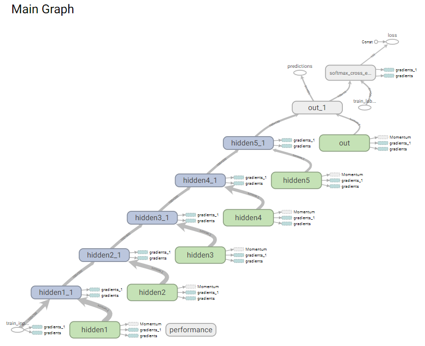
First, you will see what the computational graph of your model looks like. You can access this view by clicking on the Graphs view on in TensorBoard. It should look like the image below. You can see that you have a nice flow from train_inputs to loss and predictions flowing through the hidden layers 1 to 5.
Visualize the Summary Data
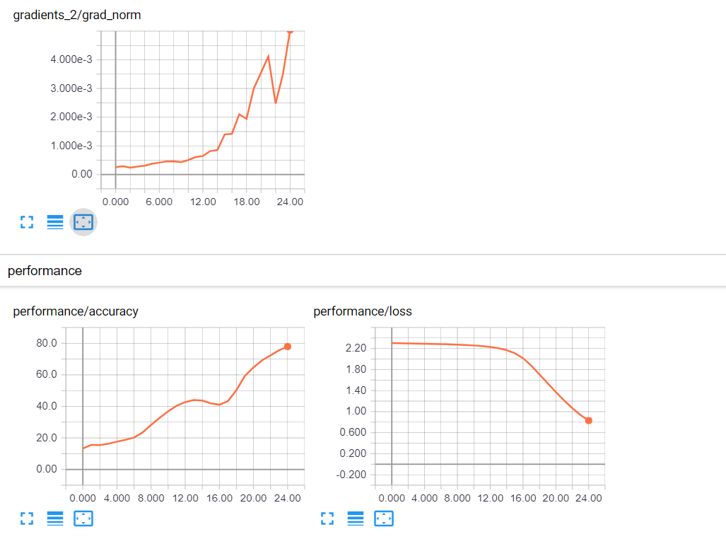
MNIST classification is one of the simplest examples, and it still cannot be solved with a 5 layer neural network. For MNIST, it's not difficult to achieve an accuracy of more than 90% in less than 5 epochs.
So what is going on here?
Let's take a look at TensorBoard:
Observations and Conclusions
You can see that the accuracy is going up, but very slowly, and that the gradient updates are increasing over time. This is an odd behavior. If you're reaching towards convergence, you should see the gradients diminishing (approaching zero), not increasing. But because the accuracy is going up, you're on the right path. You probably need a higher learning rate.
You can now try a learning rate of 0.01. This is almost identical to the previous execution of the neural network, except that you will be using 0.01 instead of 0.0001. Instead of tf_learning_rate: 0.0001, use tf_learning_rate: 0.01. Beware that there are two instances in which you will need to replace the argument.
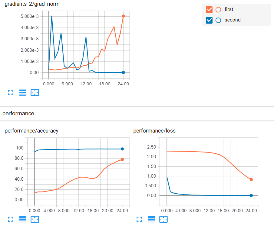
Second Look at TensorBoard: Looks Much Better Now
You can now see that the accuracy starts close to 100 and continues to go up. And you can see that the gradient updates are also diminishing over time and approaching zero. Things seems much better with the learning rate of 0.01.
Next, let's move beyond scalars. You will see how you can analyze vectors of scalars and collections of scalars.
Beyond Scalars: Visualizing Histograms/Distributions
You saw the benefit of visualizing scalars through TensorBoard, which allowed you to see how the model behaves and fix any potential issues with the model. Moreover, visualizing the graph allowed you to see that there is an uninterrupted link from the inputs to the predictions, which is necessary for gradient calculations.
Now, you're going to see another useful view in TensorBoard; histograms or distributions.
Remember that a histogram is a collection of values represented by the frequency/density that the value has in the collection. You can use histograms to visualize the network weight values over time. Visualizing network weights is important, because if the weights are wildly jumping here and there during learning, it indicates something is wrong with the weight initialization or the learning rate.
You will see how weights change in the example. If you look at the code, it uses a truncated_normal_initializer() to initialize weights.
Defining Histogram Summaries to Visualize Weights and Biases
Here you again define the tf.summary objects. However, now you are visualizing vectors of scalars so you need to define tf.summary.histogram objects.
In this case, you define two histogram objects (namely, tf_w_hist and tf_b_hist) that contain weights and biases of a given layer. You will define such histogram objects for all the layers and each layer will have its own name scope.
Finally, you can use the tf.summary.merge operation to create a grouped operation that executes all these summaries at once.
# Summaries need to be displayed
# Create a summary for each weight bias in each layer
all_summaries = []
for lid in layer_ids:
    with tf.name_scope(lid+'_hist'):
        with tf.variable_scope(lid,reuse=True):
            w,b = tf.get_variable('weights'), tf.get_variable('bias')

            # Create a scalar summary object for the loss so it can be displayed
            tf_w_hist = tf.summary.histogram('weights_hist', tf.reshape(w,[-1]))
            tf_b_hist = tf.summary.histogram('bias_hist', b)
            all_summaries.extend([tf_w_hist, tf_b_hist])

# Merge all parameter histogram summaries together
tf_param_summaries = tf.summary.merge(all_summaries)
Executing the neural network (with Histogram Summaries)
This step is almost the same as what you did before, but here you have few additional lines to compute the histogram summaries (that is, tf_param_summaries).
Note that the learning rates have also changed again.
image_size = 28
n_channels = 1
n_classes = 10
n_train = 55000
n_valid = 5000
n_test = 10000
n_epochs = 25

config = tf.ConfigProto(allow_soft_placement=True)
config.gpu_options.allow_growth = True
config.gpu_options.per_process_gpu_memory_fraction = 0.9 # making sure Tensorflow doesn't overflow the GPU

session = tf.InteractiveSession(config=config)

if not os.path.exists('summaries'):
    os.mkdir('summaries')
if not os.path.exists(os.path.join('summaries','third')):
    os.mkdir(os.path.join('summaries','third'))

summ_writer_3 = tf.summary.FileWriter(os.path.join('summaries','third'), session.graph)

tf.global_variables_initializer().run()

accuracy_per_epoch = []
mnist_data = input_data.read_data_sets('MNIST_data', one_hot=True)


for epoch in range(n_epochs):
    loss_per_epoch = []
    for i in range(n_train//batch_size):

        # =================================== Training for one step ========================================
        batch = mnist_data.train.next_batch(batch_size)    # Get one batch of training data
        if i == 0:
            # Only for the first epoch, get the summary data
            # Otherwise, it can clutter the visualization
            l,_,gn_summ, wb_summ = session.run([tf_loss,tf_loss_minimize,tf_gradnorm_summary, tf_param_summaries],
                                      feed_dict={train_inputs: batch[0].reshape(batch_size,image_size*image_size),
                                                 train_labels: batch[1],
                                                tf_learning_rate: 0.00001})
            summ_writer_3.add_summary(gn_summ, epoch)
            summ_writer_3.add_summary(wb_summ, epoch)
        else:
            # Optimize with training data
            l,_ = session.run([tf_loss,tf_loss_minimize],
                              feed_dict={train_inputs: batch[0].reshape(batch_size,image_size*image_size),
                                         train_labels: batch[1],
                                         tf_learning_rate: 0.01})
        loss_per_epoch.append(l)

    print('Average loss in epoch %d: %.5f'%(epoch,np.mean(loss_per_epoch)))
    avg_loss = np.mean(loss_per_epoch)

    # ====================== Calculate the Validation Accuracy ==========================
    valid_accuracy_per_epoch = []
    for i in range(n_valid//batch_size):
        valid_images,valid_labels = mnist_data.validation.next_batch(batch_size)
        valid_batch_predictions = session.run(
            tf_predictions,feed_dict={train_inputs: valid_images.reshape(batch_size,image_size*image_size)})
        valid_accuracy_per_epoch.append(accuracy(valid_batch_predictions,valid_labels))

    mean_v_acc = np.mean(valid_accuracy_per_epoch)
    print('\tAverage Valid Accuracy in epoch %d: %.5f'%(epoch,np.mean(valid_accuracy_per_epoch)))

    # ===================== Calculate the Test Accuracy ===============================
    accuracy_per_epoch = []
    for i in range(n_test//batch_size):
        test_images, test_labels = mnist_data.test.next_batch(batch_size)
        test_batch_predictions = session.run(
            tf_predictions,feed_dict={train_inputs: test_images.reshape(batch_size,image_size*image_size)}
        )
        accuracy_per_epoch.append(accuracy(test_batch_predictions,test_labels))

    print('\tAverage Test Accuracy in epoch %d: %.5f\n'%(epoch,np.mean(accuracy_per_epoch)))
    avg_test_accuracy = np.mean(accuracy_per_epoch)

    # Execute the summaries defined above
    summ = session.run(performance_summaries, feed_dict={tf_loss_ph:avg_loss, tf_accuracy_ph:avg_test_accuracy})

    # Write the obtained summaries to the file, so they can be displayed
    summ_writer_3.add_summary(summ, epoch)

session.close()
Extracting MNIST_data/train-images-idx3-ubyte.gz
Extracting MNIST_data/train-labels-idx1-ubyte.gz
Extracting MNIST_data/t10k-images-idx3-ubyte.gz
Extracting MNIST_data/t10k-labels-idx1-ubyte.gz
Average loss in epoch 0: 1.02625
    Average Valid Accuracy in epoch 0: 92.76000
    Average Test Accuracy in epoch 0: 92.65000

Average loss in epoch 1: 0.19110
    Average Valid Accuracy in epoch 1: 95.80000
    Average Test Accuracy in epoch 1: 95.48000

  ...
  ...
  ...

Average loss in epoch 24: 0.00009
    Average Valid Accuracy in epoch 24: 98.28000
    Average Test Accuracy in epoch 24: 98.09000
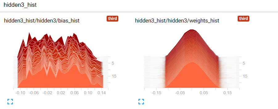
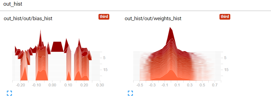
Visualizing Histogram Data of Weights and Biases
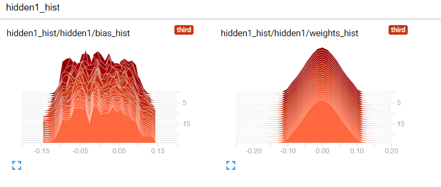
Here's what your weights and biases look like. First, you have 3 axes; time (x-axis), value (y-axis) and frequency/density of values (z-axis). Darker histograms represent older data and lighter histograms represent newer data. A higher value on the z axis means that the vector contains more values near that specific value.
Note: you also have an "overlay" view of the histograms over time as well. You can change the type of display on the left side option panel.
The Effect of Different Initializers
Now, instead of using truncated_normal_initializer(), you will use the xavier_initializer() to initialize weights. Xavier initialization is a much better initialization technique, especially for deep neural networks.
This is because instead of using a user defined standard deviation (as you did when using the truncated_normal_initializer()), Xavier initialization automatically decides the standard deviation based on the number of input and output connections to a layer. This helps to flow gradients from top to bottom without issues like vanishing gradient. You then define the model again.
First, you define a batch_size denoting the amount of data you sample at a single optimization/validation or testing step. You can then define the layer_ids, which give an identifier for each of the layers of the neural network you will be defining.
You can then define layer_sizes. Note that len(layer_sizes) should be len(layer_ids)+1, because layer_sizes includes the size of the input at the beginning. MNIST has images of size 28x28, which will be 784 when unwrapped to a single dimension.
Then, you can define the input and label placeholders, which you will later use to train the model. Finally, you define two TensorFlow variables for each layer (that is, weights and bias).
Note: This is identical to the code you used first time, except for the initialization technique used for the weights
batch_size = 100
layer_ids = ['hidden1','hidden2','hidden3','hidden4','hidden5','out']
layer_sizes = [784, 500, 400, 300, 200, 100, 10]

tf.reset_default_graph()

# Inputs and Labels
train_inputs = tf.placeholder(tf.float32, shape=[batch_size, layer_sizes[0]], name='train_inputs')
train_labels = tf.placeholder(tf.float32, shape=[batch_size, layer_sizes[-1]], name='train_labels')

# Weight and Bias definitions
for idx, lid in enumerate(layer_ids):

    with tf.variable_scope(lid):
        w = tf.get_variable('weights',shape=[layer_sizes[idx], layer_sizes[idx+1]],
                            initializer=tf.contrib.layers.xavier_initializer())
        b = tf.get_variable('bias',shape= [layer_sizes[idx+1]],
                            initializer=tf.random_uniform_initializer(-0.1,0.1))
Calculating Logits, Predictions, Loss and Optimization
With the input/output placeholders, weights and biases of each layer defined, you now can define the calculations to calculate the logits of the neural network again.
Note: This part is identical to the code you used the first time you defined these operations and tensors.
Define Summaries
Here you can define the tf.summary objects again. This is also identical to the code you used the first time you defined these operations and tensors.
Histogram Summaries: Visualizing Weights and Biases
Here you again define the tf.summary objects. However, you now are visualizing vectors of scalars so you need to define tf.summary.histogram objects.
Note that this is identical to the code you used the first time you defined these operations and tensors.
Execute the neural network
Note that this is the same as what you did before in the previous section!
There are only a few bits of code that you need to change: the three occurrences of os.path.join('summaries','third') to os.path.join('summaries','fourth'), summ_writer_3 to summ_writer_4 (this appears 4 times) and the tf_learning_rate of 0.00001 has to be set to 0.01.
image_size = 28
n_channels = 1
n_classes = 10
n_train = 55000
n_valid = 5000
n_test = 10000
n_epochs = 25

config = tf.ConfigProto(allow_soft_placement=True)
config.gpu_options.allow_growth = True
config.gpu_options.per_process_gpu_memory_fraction = 0.9 # making sure TensorFlow doesn't overflow the GPU

session = tf.InteractiveSession(config=config)

if not os.path.exists('summaries'):
    os.mkdir('summaries')
if not os.path.exists(os.path.join('summaries','fourth')):
    os.mkdir(os.path.join('summaries','fourth'))

summ_writer_4 = tf.summary.FileWriter(os.path.join('summaries','fourth'), session.graph)

tf.global_variables_initializer().run()

accuracy_per_epoch = []
mnist_data = input_data.read_data_sets('MNIST_data', one_hot=True)


for epoch in range(n_epochs):
    loss_per_epoch = []
    for i in range(n_train//batch_size):

        # =================================== Training for one step ========================================
        batch = mnist_data.train.next_batch(batch_size)    # Get one batch of training data
        if i == 0:
            # Only for the first epoch, get the summary data
            # Otherwise, it can clutter the visualization
            l,_,gn_summ, wb_summ = session.run([tf_loss,tf_loss_minimize,tf_gradnorm_summary, tf_param_summaries],
                                      feed_dict={train_inputs: batch[0].reshape(batch_size,image_size*image_size),
                                                 train_labels: batch[1],
                                                tf_learning_rate: 0.01})
            summ_writer_4.add_summary(gn_summ, epoch)
            summ_writer_4.add_summary(wb_summ, epoch)
        else:
            # Optimize with training data
            l,_ = session.run([tf_loss,tf_loss_minimize],
                              feed_dict={train_inputs: batch[0].reshape(batch_size,image_size*image_size),
                                         train_labels: batch[1],
                                         tf_learning_rate: 0.01})
        loss_per_epoch.append(l)

    print('Average loss in epoch %d: %.5f'%(epoch,np.mean(loss_per_epoch)))
    avg_loss = np.mean(loss_per_epoch)

    # ====================== Calculate the Validation Accuracy ==========================
    valid_accuracy_per_epoch = []
    for i in range(n_valid//batch_size):
        valid_images,valid_labels = mnist_data.validation.next_batch(batch_size)
        valid_batch_predictions = session.run(
            tf_predictions,feed_dict={train_inputs: valid_images.reshape(batch_size,image_size*image_size)})
        valid_accuracy_per_epoch.append(accuracy(valid_batch_predictions,valid_labels))

    mean_v_acc = np.mean(valid_accuracy_per_epoch)
    print('\tAverage Valid Accuracy in epoch %d: %.5f'%(epoch,np.mean(valid_accuracy_per_epoch)))

    # ===================== Calculate the Test Accuracy ===============================
    accuracy_per_epoch = []
    for i in range(n_test//batch_size):
        test_images, test_labels = mnist_data.test.next_batch(batch_size)
        test_batch_predictions = session.run(
            tf_predictions,feed_dict={train_inputs: test_images.reshape(batch_size,image_size*image_size)}
        )
        accuracy_per_epoch.append(accuracy(test_batch_predictions,test_labels))

    print('\tAverage Test Accuracy in epoch %d: %.5f\n'%(epoch,np.mean(accuracy_per_epoch)))
    avg_test_accuracy = np.mean(accuracy_per_epoch)

    # Execute the summaries defined above
    summ = session.run(performance_summaries, feed_dict={tf_loss_ph:avg_loss, tf_accuracy_ph:avg_test_accuracy})

    # Write the obtained summaries to the file, so they can be displayed
    summ_writer_4.add_summary(summ, epoch)

session.close()
Extracting MNIST_data/train-images-idx3-ubyte.gz
Extracting MNIST_data/train-labels-idx1-ubyte.gz
Extracting MNIST_data/t10k-images-idx3-ubyte.gz
Extracting MNIST_data/t10k-labels-idx1-ubyte.gz
Average loss in epoch 0: 0.43618
    Average Valid Accuracy in epoch 0: 95.70000
    Average Test Accuracy in epoch 0: 95.22000

Average loss in epoch 1: 0.12872
    Average Valid Accuracy in epoch 1: 96.86000
    Average Test Accuracy in epoch 1: 96.71000

  ...
  ...
  ...

Average loss in epoch 24: 0.00009
    Average Valid Accuracy in epoch 24: 98.42000
    Average Test Accuracy in epoch 24: 98.21000
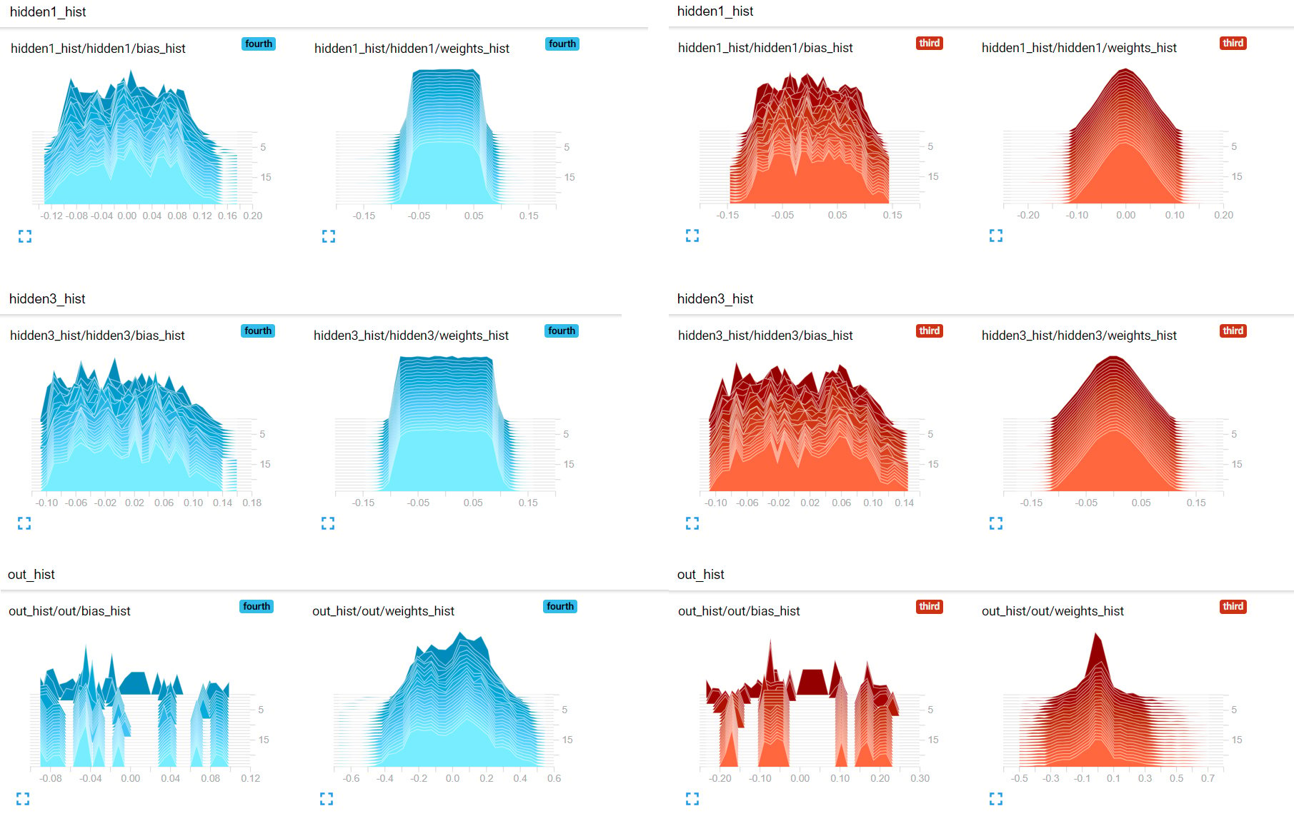
How to Compare Different Initialization Techniques
Here you can compare how weights evolve over time for the two different initalizations; truncated_normal_initializer (red) and xavier_initializer (blue). You can see that xavier_initializer keeps more weights away from zero than the normal initializer, which is a better thing to do. This is potentially allowing the Xavier initialized neural networks to converge faster, as evident by the loss/accuracy curves.
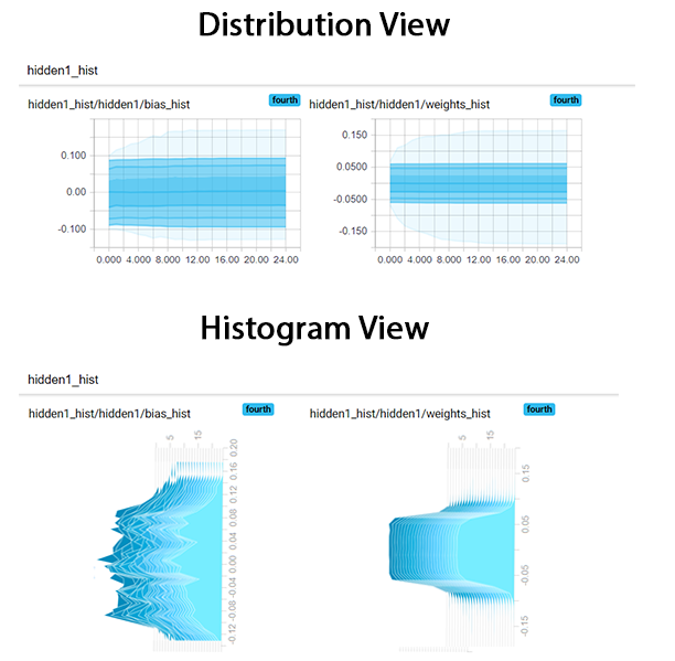
Distribution View of Histograms
You now can compare the difference between the two views; histogram view and the distribution view. Distribution view is essentially a different way of looking at the histograms. If you look at the image below, you can easily see that the distribution view is a top view of the histogram view. Note that the histogram graphs are rotated in this case to easily see the resemblance.
Conclusion
In this tutorial, you saw how to use TensorBoard. First, you learned how to start its service through the command prompt (Windows) or terminal (Ubuntu/Mac). Next, you looked at different views of data provided by TensorBoard. You then looked at code that visualizes scalar values (for example loss / accuracy) and used a feed-forward neural network model to concretely understand the use of the scalar value visualization.
Thereafter, you explored how you can visualize collections/vectors of scalars using the histogram view. This was followed by a comparison highlighting the differences between neural network weight initialization techniques using the histogram view.
Finally, you discussed the similarities between the distribution view and the histogram view.
If you would like to learn more about deep learning, be sure to take a look at our Deep Learning in Keras course.
Check out our Hyperparameter Optimization in Machine Learning Models tutorial to learn more about parameters and hyperparameters.
If you'd like to get in touch with me, you can drop me an e-mail at thushv@gmail.com or connect with me via LinkedIn.
