在自定义数据集上微调 SAM 2：教程

什么是 SAM2？

SAM2 是 Meta 开发的一个基础模型，用于图像与视频中的可提示（promptable）视觉分割。与其前身 SAM主要聚焦静态图像不同，SAM2 也被设计来处理视频分割的复杂性。

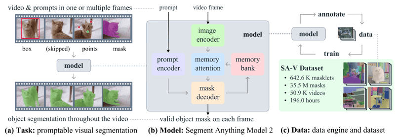
SAM2 - 任务、模型与数据（来源： Ravi 等，2024）

它采用带有流式内存的Transformer 架构，从而实现实时视频处理。SAM 2 的训练使用了海量且多样的数据集，其中包含新提出的 SA-V 数据集，涵盖超过 5.1 万个视频、60 万余条 masklet 标注。

其数据引擎支持交互式数据采集与模型改进，使模型具备“分割一切”的潜力。该引擎让 SAM 2 能持续学习与自适应，更高效地处理新颖与具挑战性的数据。然而，对于特定领域任务或稀有目标，要实现最佳表现仍需进行微调。

为什么要微调 SAM2？

在 SAM 2 的语境中，微调是指在特定数据集上对预训练的 SAM 2 模型进行进一步训练，以提升其在某个特定任务或领域上的表现。尽管 SAM 2 基于广泛多样的数据进行训练、功能强大，但其通用属性在处理专门或稀有任务时，未必总能产出最佳结果。

例如，若您正在从事一个医学影像项目，需要识别特定类型的肿瘤，由于模型训练的泛化属性，其表现可能不尽如人意。

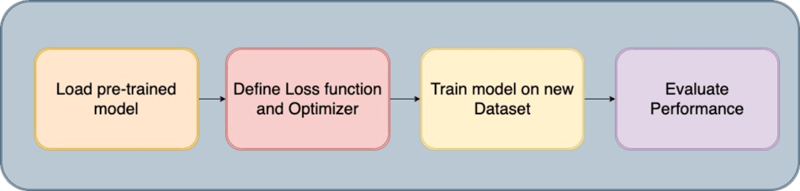
微调流程

微调 SAM 2 可以解决上述局限：它允许您让模型适配自己的数据集，从而提升模型的准确率，并让其在您的独特用例中更有效。

微调 SAM 2 的主要好处如下：

1. 提高准确性：在您的特定数据集上微调模型，可显著提升其准确率，确保在目标应用中有更佳表现。
2. 面向专门场景的分割：微调能让模型擅长分割与项目相关的特定目标类型、视觉风格或环境，产出通用模型难以实现的定制化结果。
3. 效率更高：相比从零训练，微调往往更高效，通常需要更少的数据与时间，是快速适配新任务或小众任务的务实方案。

开始微调 SAM 2：前置条件

开始微调 SAM 2，您需要准备以下条件：

1. 获取 SAM 2 模型与代码库：需要能够访问 SAM 2 模型及其代码库。您可以从Meta 的 GitHub 仓库下载预训练的 SAM 2 模型。
2. 合适的数据集：您需要包含真实分割掩码（ground truth masks）的数据集。本教程将使用Chest CT Segmentation 数据集，您可以下载并准备用于训练。
3. 计算资源：微调 SAM 2 需要具备足够算力的硬件。强烈建议使用 GPU，以保证过程高效可控，尤其在处理大型数据集或复杂模型时。本示例中在 Google Colab 上使用 A100 GPU。

软件与其他要求：

• Python 3.11 或更高版本
• PyTorch
• OpenCV：使用 !pip install opencv-python 安装

为微调 SAM 2 准备数据集

数据集质量对于微调 SAM 2 至关重要。要想得到最佳表现，高质量的、带有准确分割掩码的标注图像或视频不可或缺。精确的标注能让模型学到正确特征，从而在真实应用中获得更好的分割准确率与鲁棒性。

1. 数据获取

第一步是获取数据集，这是整个训练流程的基石。我们从Kaggle 获取数据，Kaggle 是一个提供多样数据集的可靠平台。借助 Kaggle API，我们以所需格式下载数据，确保图像与对应的分割掩码可直接用于后续处理。

2. 数据解压与清理

下载完成后，我们进行了以下步骤：

• 解压与清理： 从压缩包中解压数据，并删除不必要的文件以节省磁盘空间。
• ID 提取： 提取图像与掩码的唯一标识（ID），以确保训练中二者能正确映射。
• 移除无用文件： 删除噪声或不相关文件，例如存在已知问题的部分图像，确保数据集的完整性。

3. 转换为可用格式

由于 SAM2 模型需要特定输入格式，我们进行了如下转换：

• DICOM 转NumPy： 读取 DICOM 图像并存为 NumPy 数组，再统一调整为 512x512 的标准尺寸。
• 掩码的 NRRD 转 NumPy： 同样地，包含肺、心脏与气管掩码的 NRRD 文件被处理并保存为 NumPy 数组，然后调整形状以与对应图像匹配。
• 转换为 JPG/PNG： 为了更好的可视化与兼容性，将 NumPy 数组转换为 JPG/PNG 格式，包括对图像强度值进行归一化以及确保掩码方向正确。

4. 保存与组织数据

随后将处理后的图像与掩码分别组织到对应文件夹，以便在微调过程中便捷访问。此外，还会将这些图像与掩码的路径写入一个 CSV 文件（train.csv），以便训练时进行数据加载。

5. 可视化与验证

最后一步是验证数据集以确保其准确性：

• 可视化：通过将掩码叠加在图像上进行可视化，检查掩码的对齐与准确性。
• 抽样检查：检查若干样本，确认数据集准备无误，可用于微调。

这里提供了一个简易 notebook，带您走通数据集创建的代码。您可以按照该路径创建数据，或直接使用任意与前置条件中所述格式相同的在线数据集。

微调 SAM2

Segment Anything Model 2 包含多个组件，而更快微调的关键在于仅训练轻量组件，例如掩码解码器与提示编码器，而非整个模型。微调该模型的步骤如下：

步骤 1：安装 SAM-2

开始微调前，需要安装 SAM-2 库，这是 Segment Anything Model（SAM2）的关键依赖。该模型被设计为高效处理多种分割任务。安装方式为从 GitHub 克隆 SAM-2 仓库并安装必要依赖。

!git clone https://github.com/facebookresearch/segment-anything-2
%cd /content/segment-anything-2
!pip install -q -e .技术支持

上述代码片段可确保 SAM2 库正确安装，为我们的微调流程做好准备。

步骤 2：下载数据集

安装好 SAM-2 库后，下一步是获取用于微调的数据集。我们使用来自 Kaggle 的胸部 CT 分割数据集，其中包含肺、心脏与气管的图像与掩码。

数据集包含：

• images.zip：RGB 格式的图像
• masks.zip：RGB 格式的分割掩码
• train.csv：包含图像名称的 CSV 文件

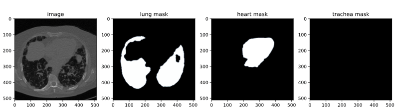
CT 扫描数据集中的图像

在本文中，我们只使用肺部的图像与掩码进行分割。Kaggle API 允许我们将数据集直接下载到运行环境。首先从 Kaggle 上传 kaggle.json 文件，以便轻松访问任意数据集。

获取 kaggle.json 的方法：进入您个人资料下的 Settings 选项卡，选择 Create New Token。这将触发下载 kaggle.json，该文件包含您的 API 凭据。

# get dataset from Kaggle
from google.colab import files
files.upload()  # This will prompt you to upload the kaggle.json file

!mkdir -p ~/.kaggle
!mv kaggle.json ~/.kaggle/
!chmod 600 ~/.kaggle/kaggle.json
!kaggle datasets download -d polomarco/chest-ct-segmentation技术支持

解压数据：

!unzip chest-ct-segmentation.zip -d chest-ct-segmentation技术支持

数据集准备就绪后，就可以开始微调流程。如前所述，关键在于仅微调 SAM2 的轻量组件，如掩码解码器与提示编码器，而非整个模型。此方法更高效，也更省资源。

步骤 3：下载 SAM-2 检查点

微调需要从预训练的 SAM2 模型权重开始。这些权重称为“检查点（checkpoints）”，是进一步训练的起点。检查点已在大量多样图像上训练，通过在我们的特定数据集上微调，可在目标任务上获得更好的表现。

!wget -O sam2_hiera_tiny.pt "https://dl.fbaipublicfiles.com/segment_anything_2/072824/sam2_hiera_tiny.pt"
!wget -O sam2_hiera_small.pt "https://dl.fbaipublicfiles.com/segment_anything_2/072824/sam2_hiera_small.pt"
!wget -O sam2_hiera_base_plus.pt "https://dl.fbaipublicfiles.com/segment_anything_2/072824/sam2_hiera_base_plus.pt"
!wget -O sam2_hiera_large.pt "https://dl.fbaipublicfiles.com/segment_anything_2/072824/sam2_hiera_large.pt"技术支持

在此步骤中，我们下载不同大小（如 tiny、small、base_plus、large）的 SAM-2 检查点。可根据可用算力与具体任务选择合适的检查点。

步骤 4：数据准备

下载数据集后，下一步是为训练做准备。包括将数据集划分为训练集与测试集，并创建可在微调过程中馈入 SAM 2 模型的数据结构。

%cd /content/segment-anything-2

import os
import pandas as pd
import cv2
import torch
import torch.nn.utils
import numpy as np
import matplotlib.pyplot as plt
import matplotlib.colors as mcolors
from sklearn.model_selection import train_test_split
from sam2.build_sam import build_sam2
from sam2.sam2_image_predictor import SAM2ImagePredictor

# Path to the chest-ct-segmentation dataset folder
data_dir = "/content/segment-anything-2/chest-ct-segmentation"
images_dir = os.path.join(data_dir, "images/images")
masks_dir = os.path.join(data_dir, "masks/masks")

# Load the train.csv file
train_df = pd.read_csv(os.path.join(data_dir, "train.csv"))

# Split the data into two halves: one for training and one for testing
train_df, test_df = train_test_split(train_df, test_size=0.2, random_state=42)

# Prepare the training data list
train_data = []
for index, row in train_df.iterrows():
   image_name = row['ImageId']
   mask_name = row['MaskId']

   # Append image and corresponding mask paths
   train_data.append({
       "image": os.path.join(images_dir, image_name),
       "annotation": os.path.join(masks_dir, mask_name)
   })

# Prepare the testing data list (if needed for inference or evaluation later)
test_data = []
for index, row in test_df.iterrows():
   image_name = row['ImageId']
   mask_name = row['MaskId']

   # Append image and corresponding mask paths
   test_data.append({
       "image": os.path.join(images_dir, image_name),
       "annotation": os.path.join(masks_dir, mask_name)
   })
技术支持

我们将数据集按 80%/20% 划分为训练集与测试集，以便在训练后评估模型表现。训练数据用于微调 SAM 2，测试数据用于推理与评估。

在完成训练/测试划分后，接下来要创建二值掩码、在这些掩码内选择关键点，并进行可视化，以确保数据被正确处理。

1. 读取与缩放图像：流程从随机选取一个图像及其对应掩码开始。图像从 BGR 转为 RGB 格式，这是大多数深度学习模型的标准色彩格式。对应标注（掩码）以灰度模式读取。随后，将图像与标注掩码按最长边不超过 1024 像素等比例缩放，以满足模型输入要求并降低计算负担。

def read_batch(data, visualize_data=False):
   # Select a random entry
   ent = data[np.random.randint(len(data))]

   # Get full paths
   Img = cv2.imread(ent["image"])[..., ::-1]  # Convert BGR to RGB
   ann_map = cv2.imread(ent["annotation"], cv2.IMREAD_GRAYSCALE)  # Read annotation as grayscale

   if Img is None or ann_map is None:
       print(f"Error: Could not read image or mask from path {ent['image']} or {ent['annotation']}")
       return None, None, None, 0

   # Resize image and mask
   r = np.min([1024 / Img.shape[1], 1024 / Img.shape[0]])  # Scaling factor
   Img = cv2.resize(Img, (int(Img.shape[1] * r), int(Img.shape[0] * r)))
   ann_map = cv2.resize(ann_map, (int(ann_map.shape[1] * r), int(ann_map.shape[0] * r)), interpolation=cv2.INTER_NEAREST)
技术支持

2. 分割掩码二值化：将多类别标注掩码（不同像素值标注不同目标）转换为二值掩码，该掩码突出图像中的所有兴趣区域，将分割问题简化为二分类（目标 vs. 背景）。随后使用 5x5 卷积核对二值掩码进行腐蚀处理。

腐蚀会略微缩小掩码，以避免在选择点时出现边界效应，确保所选点位于目标内部，而非接近噪声或不确定的边缘。

接着从腐蚀后的掩码内部选择关键点。这些点在微调过程中作为提示，引导模型关注重点区域。点从目标内部随机采样，以具代表性并减少边界噪声影响。

   ### Continuation of read_batch() ###

   # Initialize a single binary mask
   binary_mask = np.zeros_like(ann_map, dtype=np.uint8)
   points = []

   # Get binary masks and combine them into a single mask
   inds = np.unique(ann_map)[1:]  # Skip the background (index 0)
   for ind in inds:
       mask = (ann_map == ind).astype(np.uint8)  # Create binary mask for each unique index
       binary_mask = np.maximum(binary_mask, mask)  # Combine with the existing binary mask

   # Erode the combined binary mask to avoid boundary points
   eroded_mask = cv2.erode(binary_mask, np.ones((5, 5), np.uint8), iterations=1)

   # Get all coordinates inside the eroded mask and choose a random point
   coords = np.argwhere(eroded_mask > 0)
   if len(coords) > 0:
       for _ in inds:  # Select as many points as there are unique labels
           yx = np.array(coords[np.random.randint(len(coords))])
           points.append([yx[1], yx[0]])

   points = np.array(points)
技术支持

3. 可视化：此步骤用于核验预处理是否正确。通过在二值掩码上可视化这些点，您可以确保模型在训练时将获得合适的输入。最后，将二值掩码按模型输入的维度正确重塑与格式化，同时也重塑这些点，以便在后续训练中使用。函数会返回处理后的图像、二值掩码、所选点以及掩码数量。

    ### Continuation of read_batch() ###

    if visualize_data:
        # Plotting the images and points
        plt.figure(figsize=(15, 5))

        # Original Image
        plt.subplot(1, 3, 1)
        plt.title('Original Image')
        plt.imshow(img)
        plt.axis('off')

        # Segmentation Mask (binary_mask)
        plt.subplot(1, 3, 2)
        plt.title('Binarized Mask')
        plt.imshow(binary_mask, cmap='gray')
        plt.axis('off')

        # Mask with Points in Different Colors
        plt.subplot(1, 3, 3)
        plt.title('Binarized Mask with Points')
        plt.imshow(binary_mask, cmap='gray')

        # Plot points in different colors
        colors = list(mcolors.TABLEAU_COLORS.values())
        for i, point in enumerate(points):
            plt.scatter(point[0], point[1], c=colors[i % len(colors)], s=100, label=f'Point {i+1}')  # Corrected to plot y, x order

        # plt.legend()
        plt.axis('off')

        plt.tight_layout()
        plt.show()

    binary_mask = np.expand_dims(binary_mask, axis=-1)  # Now shape is (1024, 1024, 1)
    binary_mask = binary_mask.transpose((2, 0, 1))
    points = np.expand_dims(points, axis=1)

    # Return the image, binarized mask, points, and number of masks
    return img, binary_mask, points, len(inds)

# Visualize the data
Img1, masks1, points1, num_masks = read_batch(train_data, visualize_data=True)
技术支持

上述代码会返回如下图：包含原始图像、其二值掩码，以及带有点的二值掩码。

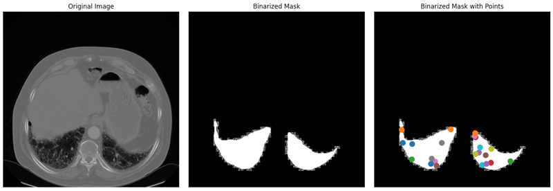
数据集的原始图像、二值掩码与带点的二值掩码。

步骤 5：微调 SAM2 模型

微调 SAM2 模型包含多个步骤，包括加载模型、设置优化器与调度器，并基于训练数据迭代更新模型权重。

加载模型检查点：

sam2_checkpoint = "sam2_hiera_small.pt"  # @param ["sam2_hiera_tiny.pt", "sam2_hiera_small.pt", "sam2_hiera_base_plus.pt", "sam2_hiera_large.pt"]
model_cfg = "sam2_hiera_s.yaml" # @param ["sam2_hiera_t.yaml", "sam2_hiera_s.yaml", "sam2_hiera_b+.yaml", "sam2_hiera_l.yaml"]

sam2_model = build_sam2(model_cfg, sam2_checkpoint, device="cuda")
predictor = SAM2ImagePredictor(sam2_model)
技术支持

我们首先基于预训练检查点构建 SAM2 模型。随后将模型封装进预测器类，便于设置图像、编码提示与解码掩码。

配置超参数

我们配置若干超参数以确保模型有效学习，比如学习率、权重衰减与梯度累积步数。它们控制学习过程，包括权重更新速度与防止过拟合的机制。您可根据需要自行调整。

# Train mask decoder.
predictor.model.sam_mask_decoder.train(True)

# Train prompt encoder.
predictor.model.sam_prompt_encoder.train(True)

# Configure optimizer.
optimizer=torch.optim.AdamW(params=predictor.model.parameters(),lr=0.0001,weight_decay=1e-4) #1e-5, weight_decay = 4e-5

# Mix precision.
scaler = torch.cuda.amp.GradScaler()

# No. of steps to train the model.
NO_OF_STEPS = 3000 # @param 

# Fine-tuned model name.
FINE_TUNED_MODEL_NAME = "fine_tuned_sam2"
技术支持

优化器负责更新模型权重，调度器在训练过程中调整学习率以改进收敛。通过合理微调这些参数，可以获得更好的分割准确率。

开始训练

微调过程是迭代式的：每一步都会将仅包含肺部的图像与掩码批量输入模型，计算损失并用于更新权重。

# Initialize scheduler
scheduler = torch.optim.lr_scheduler.StepLR(optimizer, step_size=500, gamma=0.2) # 500 , 250, gamma = 0.1
accumulation_steps = 4  # Number of steps to accumulate gradients before updating

for step in range(1, NO_OF_STEPS + 1):
   with torch.cuda.amp.autocast():
       image, mask, input_point, num_masks = read_batch(train_data, visualize_data=False)
       if image is None or mask is None or num_masks == 0:
           continue

       input_label = np.ones((num_masks, 1))
       if not isinstance(input_point, np.ndarray) or not isinstance(input_label, np.ndarray):
           continue

       if input_point.size == 0 or input_label.size == 0:
           continue

       predictor.set_image(image)
       mask_input, unnorm_coords, labels, unnorm_box = predictor._prep_prompts(input_point, input_label, box=None, mask_logits=None, normalize_coords=True)
       if unnorm_coords is None or labels is None or unnorm_coords.shape[0] == 0 or labels.shape[0] == 0:
           continue

       sparse_embeddings, dense_embeddings = predictor.model.sam_prompt_encoder(
           points=(unnorm_coords, labels), boxes=None, masks=None,
       )

       batched_mode = unnorm_coords.shape[0] > 1
       high_res_features = [feat_level[-1].unsqueeze(0) for feat_level in predictor._features["high_res_feats"]]
       low_res_masks, prd_scores, _, _ = predictor.model.sam_mask_decoder(
           image_embeddings=predictor._features["image_embed"][-1].unsqueeze(0),
           image_pe=predictor.model.sam_prompt_encoder.get_dense_pe(),
           sparse_prompt_embeddings=sparse_embeddings,
           dense_prompt_embeddings=dense_embeddings,
           multimask_output=True,
           repeat_image=batched_mode,
           high_res_features=high_res_features,
       )
       prd_masks = predictor._transforms.postprocess_masks(low_res_masks, predictor._orig_hw[-1])

       gt_mask = torch.tensor(mask.astype(np.float32)).cuda()
       prd_mask = torch.sigmoid(prd_masks[:, 0])
       seg_loss = (-gt_mask * torch.log(prd_mask + 0.000001) - (1 - gt_mask) * torch.log((1 - prd_mask) + 0.00001)).mean()

       inter = (gt_mask * (prd_mask > 0.5)).sum(1).sum(1)
       iou = inter / (gt_mask.sum(1).sum(1) + (prd_mask > 0.5).sum(1).sum(1) - inter)
       score_loss = torch.abs(prd_scores[:, 0] - iou).mean()
       loss = seg_loss + score_loss * 0.05

       # Apply gradient accumulation
       loss = loss / accumulation_steps
       scaler.scale(loss).backward()

       # Clip gradients
       torch.nn.utils.clip_grad_norm_(predictor.model.parameters(), max_norm=1.0)

       if step % accumulation_steps == 0:
           scaler.step(optimizer)
           scaler.update()
           predictor.model.zero_grad()

       # Update scheduler
       scheduler.step()

       if step % 500 == 0:
           FINE_TUNED_MODEL = FINE_TUNED_MODEL_NAME + "_" + str(step) + ".torch"
           torch.save(predictor.model.state_dict(), FINE_TUNED_MODEL)

       if step == 1:
           mean_iou = 0

       mean_iou = mean_iou * 0.99 + 0.01 * np.mean(iou.cpu().detach().numpy())

       if step % 100 == 0:
           print("Step " + str(step) + ":\t", "Accuracy (IoU) = ", mean_iou)
技术支持

在每次迭代中，模型处理一批图像，生成分割掩码并与真实值对比计算损失。随后使用该损失来调整模型权重，使其性能逐步提升。经过约 3000 个 epoch 训练，我们获得约 72% 的准确率（IoU，交并比）。

步骤 6：使用微调模型进行推理

随后可使用模型在新的、未见过的图像上进行推理，预测分割掩码。先使用 read_images 与 get_points 辅助函数，获取推理用图像及其掩码与关键点。

def read_image(image_path, mask_path):  # read and resize image and mask
   img = cv2.imread(image_path)[..., ::-1]  # Convert BGR to RGB
   mask = cv2.imread(mask_path, 0)
   r = np.min([1024 / img.shape[1], 1024 / img.shape[0]])
   img = cv2.resize(img, (int(img.shape[1] * r), int(img.shape[0] * r)))
   mask = cv2.resize(mask, (int(mask.shape[1] * r), int(mask.shape[0] * r)), interpolation=cv2.INTER_NEAREST)
   return img, mask

def get_points(mask, num_points):  # Sample points inside the input mask
   points = []
   coords = np.argwhere(mask > 0)
   for i in range(num_points):
       yx = np.array(coords[np.random.randint(len(coords))])
       points.append([[yx[1], yx[0]]])
   return np.array(points)技术支持

随后加载要推理的样例图像与新微调的权重，并在torch.no_grad() 下执行推理。

# Randomly select a test image from the test_data
selected_entry = random.choice(test_data)
image_path = selected_entry['image']
mask_path = selected_entry['annotation']

# Load the selected image and mask
image, mask = read_image(image_path, mask_path)

# Generate random points for the input
num_samples = 30  # Number of points per segment to sample
input_points = get_points(mask, num_samples)

# Load the fine-tuned model
FINE_TUNED_MODEL_WEIGHTS = "fine_tuned_sam2_1000.torch"
sam2_model = build_sam2(model_cfg, sam2_checkpoint, device="cuda")

# Build net and load weights
predictor = SAM2ImagePredictor(sam2_model)
predictor.model.load_state_dict(torch.load(FINE_TUNED_MODEL_WEIGHTS))

# Perform inference and predict masks
with torch.no_grad():
   predictor.set_image(image)
   masks, scores, logits = predictor.predict(
       point_coords=input_points,
       point_labels=np.ones([input_points.shape[0], 1])
   )

# Process the predicted masks and sort by scores
np_masks = np.array(masks[:, 0])
np_scores = scores[:, 0]
sorted_masks = np_masks[np.argsort(np_scores)][::-1]

# Initialize segmentation map and occupancy mask
seg_map = np.zeros_like(sorted_masks[0], dtype=np.uint8)
occupancy_mask = np.zeros_like(sorted_masks[0], dtype=bool)

# Combine masks to create the final segmentation map
for i in range(sorted_masks.shape[0]):
   mask = sorted_masks[i]
   if (mask * occupancy_mask).sum() / mask.sum() > 0.15:
       continue

   mask_bool = mask.astype(bool)
   mask_bool[occupancy_mask] = False  # Set overlapping areas to False in the mask
   seg_map[mask_bool] = i + 1  # Use boolean mask to index seg_map
   occupancy_mask[mask_bool] = True  # Update occupancy_mask

# Visualization: Show the original image, mask, and final segmentation side by side
plt.figure(figsize=(18, 6))

plt.subplot(1, 3, 1)
plt.title('Test Image')
plt.imshow(image)
plt.axis('off')

plt.subplot(1, 3, 2)
plt.title('Original Mask')
plt.imshow(mask, cmap='gray')
plt.axis('off')

plt.subplot(1, 3, 3)
plt.title('Final Segmentation')
plt.imshow(seg_map, cmap='jet')
plt.axis('off')

plt.tight_layout()
plt.show()技术支持

在此步骤中，我们使用微调后的模型为测试图像生成分割掩码。随后将预测掩码与原始图像及真实掩码并排可视化，以评估模型表现。

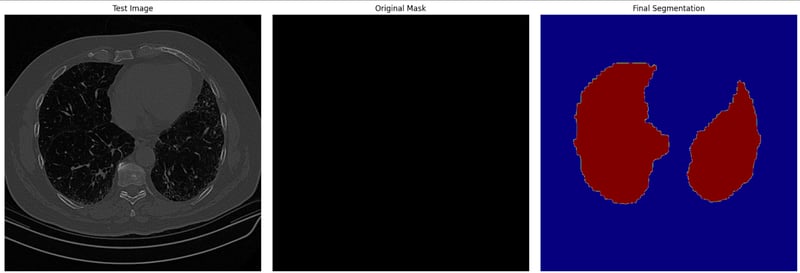
测试数据上的最终分割图像

结语

微调 SAM2 是增强其在特定任务上能力的务实方法。无论您从事医学影像、自动驾驶还是视频编辑，微调都能让 SAM2 更好地服务于您的独特需求。按照本指南，您可以将 SAM2 应用于项目中，并获得业界领先的分割效果。

对于更高级的用例，您也可以考虑微调 SAM2 的更多组件，例如图像编码器。虽然这需要更多资源，但可带来更高的灵活性与性能提升。