Fine-Tuning SAM 2 on a Custom Dataset: Tutorial

What Is SAM2?

SAM2 is a foundation model developed by Meta for promptable visual segmentation in images and videos. Unlike its predecessor, SAM, which primarily focused on static images, SAM2 is designed to handle the complexities of video segmentation as well.

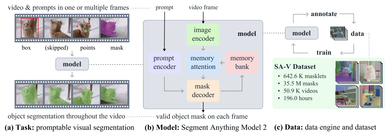
SAM2 - Task, Model, and Data (Source: Ravi et al., 2024)

It employs a transformer architecture with streaming memory, enabling real-time video processing. SAM 2's training involved a vast and varied dataset featuring the novel SA-V dataset, which includes more than 600,000 masklet annotations spanning 51,000 videos.

Its data engine, which allows for interactive data collection and model improvement, gives the model the ability to segment anything possible. This engine enables SAM 2 to continuously learn and adapt, making it more efficient at handling new and challenging data. However, for domain-specific tasks or rare objects, fine-tuning is essential to achieve optimal performance.

Why Fine-Tune SAM2?

In the context of SAM 2, fine-tuning is the process of further training the pre-trained SAM 2 model on a specific dataset to enhance its performance for a particular task or domain. While SAM 2 is a powerful tool trained on a broad and diverse dataset, its general-purpose nature may not always yield optimal results for specialized or rare tasks.

For example, if you're working on a medical imaging project that requires the identification of specific tumor types, the model's performance might fall short due to its generalized training.

The fine-tuning process

Fine-tuning SAM 2 addresses this limitation by allowing you to adapt the model to your specific dataset. This process improves the model's accuracy and makes it more effective for your unique use case.

Here are the key benefits of fine-tuning SAM 2:

1. Improved accuracy: By fine-tuning the model on your specific dataset, you can significantly enhance its accuracy, ensuring better performance in your targeted application.
2. Specialized segmentation: Fine-tuning enables the model to become adept at segmenting specific object types, visual styles, or environments that are relevant to your project, providing tailored results that a general-purpose model may not achieve.
3. Efficiency: Fine-tuning is often more efficient than training a model from scratch. It typically requires less data and time, making it a practical solution for quickly adapting the model to new or niche tasks.

Getting Started With Fine-Tuning SAM 2: Prerequisites

To get started with fine-tuning SAM 2, you’ll need to have the following prerequisites in place:

1. Access to the SAM 2 model and codebase: Have access to the SAM 2 model and its codebase. You can download the pre-trained SAM 2 model from Meta's GitHub repository.
2. A suitable dataset: You'll need a dataset that includes ground truth segmentation masks. For this tutorial, we’ll be using the Chest CT Segmentation dataset, which you can download and prepare for training.
3. Computational resources: Fine-tuning SAM 2 requires hardware with sufficient computational power. GPUs are highly recommended to ensure the process is efficient and manageable, especially when working with large datasets or complex models. In this example, an A100 GPU on Google Colab is used.

Software and other requirements:

• Python 3.11 or higher
• PyTorch
• OpenCV: Install it using !pip install opencv-python

Preparing the Dataset for Fine-Tuning SAM 2

The quality of your dataset is crucial for fine-tuning the SAM 2 model. High-quality annotated images or videos with accurate segmentation masks are essential to achieving optimal performance. Precise annotations enable the model to learn the correct features, leading to better segmentation accuracy and robustness in real-world applications.

1. Data acquisition

The first step involves acquiring the dataset, which forms the backbone of the training process. We sourced our data from Kaggle, a reliable platform that provides a diverse range of datasets. Using the Kaggle API, we downloaded the data in the required format, ensuring that the images and corresponding segmentation masks were readily available for further processing.

2. Data extraction and cleaning

After downloading the datasets, we performed the following steps:

• Unzipping and cleaning: Extract the data from the downloaded zip files and delete unnecessary files to save disk space.
• ID extraction: Unique identifiers (IDs) for images and masks are extracted to ensure correct mapping between them during training.
• Removing unnecessary files: Remove any noisy or irrelevant files, such as certain images with known issues, to maintain the integrity of the dataset.

3. Conversion to usable formats

Since the SAM2 model requires input in specific formats, we converted the data as follows:

• DICOM to NumPy: The DICOM images were read and stored as NumPy arrays, which were then resized to a standard dimension of 512x512 pixels.
• NRRD to NumPy for masks: Similarly, NRRD files containing masks for lungs, heart, and trachea were processed and saved as NumPy arrays. These masks were then reshaped to match the corresponding images.
• Conversion to JPG/PNG: For better visualization and compatibility, the NumPy arrays were converted to JPG/PNG formats. This step included normalizing the image intensity values and ensuring the masks were correctly oriented.

4. Saving and organizing data

The processed images and masks are then organized into respective folders for easy access during the fine-tuning process. Additionally, paths to these images and masks are written into a CSV file (train.csv) to facilitate data loading during training.

5. Visualization and validation

The final step involved validating the dataset to ensure its accuracy:

• Visualization: We visualized the image-mask pairs by overlaying the masks on the images. This helped us check the alignment and accuracy of the masks.
• Inspection: By inspecting a few samples, we could confirm that the dataset was correctly prepared and ready for use in fine-tuning.

Here is a quick notebook to take you through code for dataset creation. You can either go through this data creation path or directly use any dataset available online in the same format as the one mentioned in the pre-requisites.

Fine-Tuning SAM2

Segment Anything Model 2 contains several components, but the catch here for faster fine-tuning is to train only lightweight components, such as the mask decoder and prompt encoder, rather than the entire model. The steps for fine-tuning this model are as follows:

Step 1: Install SAM-2

To start the fine-tuning process, we need to install the SAM-2 library, which is crucial for the Segment Anything Model (SAM2). This model is designed to handle various segmentation tasks effectively. The installation involves cloning the SAM-2 repository from GitHub and installing the necessary dependencies.

!git clone https://github.com/facebookresearch/segment-anything-2
%cd /content/segment-anything-2
!pip install -q -e .

This code snippet ensures the SAM2 library is correctly installed and ready for use in our fine-tuning workflow.

Step 2: Download the dataset

Once the SAM-2 library is installed, the next step is to acquire the dataset we’ll be using for fine-tuning. We use a dataset available on Kaggle, specifically a chest CT segmentation dataset containing images and masks of lungs, heart, and trachea.

The dataset contains:

• images.zip: Images in RGB format
• masks.zip: Segmentation masks in RGB format
• train.csv: CSV file with image names

Image from the CT Scan Dataset

In this blog, we’ll use only images and masks of lungs for segmentation. The Kaggle API allows us to download datasets directly to our environment. We start by uploading the kaggle.json file from Kaggle to access any dataset easily.

To get kaggle.json, go to the Settings tab under your user profile and select Create New Token. This will trigger the Kaggle download. json, a file containing your API credentials.

# get dataset from Kaggle
from google.colab import files
files.upload()  # This will prompt you to upload the kaggle.json file

!mkdir -p ~/.kaggle
!mv kaggle.json ~/.kaggle/
!chmod 600 ~/.kaggle/kaggle.json
!kaggle datasets download -d polomarco/chest-ct-segmentation

Unzip the data:

!unzip chest-ct-segmentation.zip -d chest-ct-segmentation

With the dataset ready, let’s start the fine-tuning process. As I previously mentioned, the key here is to fine-tune only the lightweight components of SAM2, such as the mask decoder and prompt encoder, rather than the entire model. This approach is more efficient and requires fewer resources.

Step 3: Download SAM-2 checkpoints

For the fine-tuning process, we need to start with pre-trained SAM2 model weights. These weights, called "checkpoints," are the starting point for further training. The checkpoints have been trained on a wide range of images, and by fine-tuning them on our specific dataset, we can achieve better performance on our target tasks.

!wget -O sam2_hiera_tiny.pt "https://dl.fbaipublicfiles.com/segment_anything_2/072824/sam2_hiera_tiny.pt"
!wget -O sam2_hiera_small.pt "https://dl.fbaipublicfiles.com/segment_anything_2/072824/sam2_hiera_small.pt"
!wget -O sam2_hiera_base_plus.pt "https://dl.fbaipublicfiles.com/segment_anything_2/072824/sam2_hiera_base_plus.pt"
!wget -O sam2_hiera_large.pt "https://dl.fbaipublicfiles.com/segment_anything_2/072824/sam2_hiera_large.pt"

In this step, we download various SAM-2 checkpoints that correspond to different model sizes (e.g., tiny, small, base_plus, large). The choice of checkpoint can be adjusted based on the computational resources available and the specific task at hand.

Step 4: Data preparation

With the dataset downloaded, the next step is to prepare it for training. This involves splitting the dataset into training and testing sets and creating data structures that can be fed into the SAM 2 model during fine-tuning.

%cd /content/segment-anything-2

import os
import pandas as pd
import cv2
import torch
import torch.nn.utils
import numpy as np
import matplotlib.pyplot as plt
import matplotlib.colors as mcolors
from sklearn.model_selection import train_test_split
from sam2.build_sam import build_sam2
from sam2.sam2_image_predictor import SAM2ImagePredictor

# Path to the chest-ct-segmentation dataset folder
data_dir = "/content/segment-anything-2/chest-ct-segmentation"
images_dir = os.path.join(data_dir, "images/images")
masks_dir = os.path.join(data_dir, "masks/masks")

# Load the train.csv file
train_df = pd.read_csv(os.path.join(data_dir, "train.csv"))

# Split the data into two halves: one for training and one for testing
train_df, test_df = train_test_split(train_df, test_size=0.2, random_state=42)

# Prepare the training data list
train_data = []
for index, row in train_df.iterrows():
   image_name = row['ImageId']
   mask_name = row['MaskId']

   # Append image and corresponding mask paths
   train_data.append({
       "image": os.path.join(images_dir, image_name),
       "annotation": os.path.join(masks_dir, mask_name)
   })

# Prepare the testing data list (if needed for inference or evaluation later)
test_data = []
for index, row in test_df.iterrows():
   image_name = row['ImageId']
   mask_name = row['MaskId']

   # Append image and corresponding mask paths
   test_data.append({
       "image": os.path.join(images_dir, image_name),
       "annotation": os.path.join(masks_dir, mask_name)
   })

We split the dataset into a training set (80%) and a testing set (20%) to ensure that we can evaluate the model's performance after training. The training data will be used to fine-tune the SAM 2 model, while the testing data will be used for inference and evaluation.

After splitting your dataset into training and testing sets, the next step involves creating binary masks, selecting key points within these masks, and visualizing these elements to ensure the data is correctly processed. 

1. Reading and resizing images: The process starts by randomly selecting an image and its corresponding mask from the dataset. The image is converted from BGR to RGB format, which is the standard color format for most deep learning models. The corresponding annotation (mask) is read in grayscale mode. Then, both the image and the annotation mask are resized to a maximum dimension of 1024 pixels, maintaining the aspect ratio to ensure that the data fits within the model's input requirements and reduces computational load.

def read_batch(data, visualize_data=False):
   # Select a random entry
   ent = data[np.random.randint(len(data))]

   # Get full paths
   Img = cv2.imread(ent["image"])[..., ::-1]  # Convert BGR to RGB
   ann_map = cv2.imread(ent["annotation"], cv2.IMREAD_GRAYSCALE)  # Read annotation as grayscale

   if Img is None or ann_map is None:
       print(f"Error: Could not read image or mask from path {ent['image']} or {ent['annotation']}")
       return None, None, None, 0

   # Resize image and mask
   r = np.min([1024 / Img.shape[1], 1024 / Img.shape[0]])  # Scaling factor
   Img = cv2.resize(Img, (int(Img.shape[1] * r), int(Img.shape[0] * r)))
   ann_map = cv2.resize(ann_map, (int(ann_map.shape[1] * r), int(ann_map.shape[0] * r)), interpolation=cv2.INTER_NEAREST)

2. Binarization of segmentation masks: The multi-class annotation mask (which might have multiple object classes labeled with different pixel values) is converted into a binary mask. This mask highlights all the regions of interest in the image, simplifying the segmentation task to a binary classification problem: object vs. background. The binary mask is then eroded using a 5x5 kernel.

Erosion slightly reduces the mask's size, which helps avoid boundary effects when selecting points. This ensures the selected points are well within the object's interior rather than near its edges, which might be noisy or ambiguous.

Key points are selected from within the eroded mask. These points act as prompts during the fine-tuning process, guiding the model on where to focus its attention. The points are selected randomly from the interior of the objects to ensure they are representative and not influenced by noisy boundaries.

   ### Continuation of read_batch() ###

   # Initialize a single binary mask
   binary_mask = np.zeros_like(ann_map, dtype=np.uint8)
   points = []

   # Get binary masks and combine them into a single mask
   inds = np.unique(ann_map)[1:]  # Skip the background (index 0)
   for ind in inds:
       mask = (ann_map == ind).astype(np.uint8)  # Create binary mask for each unique index
       binary_mask = np.maximum(binary_mask, mask)  # Combine with the existing binary mask

   # Erode the combined binary mask to avoid boundary points
   eroded_mask = cv2.erode(binary_mask, np.ones((5, 5), np.uint8), iterations=1)

   # Get all coordinates inside the eroded mask and choose a random point
   coords = np.argwhere(eroded_mask > 0)
   if len(coords) > 0:
       for _ in inds:  # Select as many points as there are unique labels
           yx = np.array(coords[np.random.randint(len(coords))])
           points.append([yx[1], yx[0]])

   points = np.array(points)

3. Visualization: This step is crucial for verifying that the data preprocessing steps have been executed correctly. By visually inspecting the points on the binarized mask, you can ensure that the model will receive appropriate input during training. Finally, the binary mask is reshaped and formatted correctly (with dimensions suitable for the model input), and the points are also reshaped for further use in the training process. The function returns the processed image, binary mask, selected points, and the number of masks found.

    ### Continuation of read_batch() ###

    if visualize_data:
        # Plotting the images and points
        plt.figure(figsize=(15, 5))

        # Original Image
        plt.subplot(1, 3, 1)
        plt.title('Original Image')
        plt.imshow(img)
        plt.axis('off')

        # Segmentation Mask (binary_mask)
        plt.subplot(1, 3, 2)
        plt.title('Binarized Mask')
        plt.imshow(binary_mask, cmap='gray')
        plt.axis('off')

        # Mask with Points in Different Colors
        plt.subplot(1, 3, 3)
        plt.title('Binarized Mask with Points')
        plt.imshow(binary_mask, cmap='gray')

        # Plot points in different colors
        colors = list(mcolors.TABLEAU_COLORS.values())
        for i, point in enumerate(points):
            plt.scatter(point[0], point[1], c=colors[i % len(colors)], s=100, label=f'Point {i+1}')  # Corrected to plot y, x order

        # plt.legend()
        plt.axis('off')

        plt.tight_layout()
        plt.show()

    binary_mask = np.expand_dims(binary_mask, axis=-1)  # Now shape is (1024, 1024, 1)
    binary_mask = binary_mask.transpose((2, 0, 1))
    points = np.expand_dims(points, axis=1)

    # Return the image, binarized mask, points, and number of masks
    return img, binary_mask, points, len(inds)

# Visualize the data
Img1, masks1, points1, num_masks = read_batch(train_data, visualize_data=True)

The above code returns the following figure containing the original image from the dataset along with its binarized mask and binarized mask with points. 

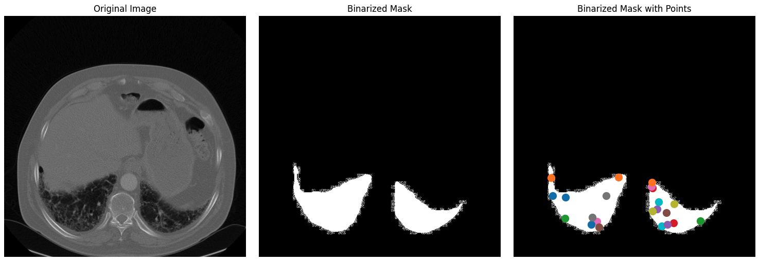
Original image, binarized mask, and binarized mask with points for the dataset.

Step 5: Fine-tuning the SAM2 model

Fine-tuning the SAM2 model involves several steps, including loading the model, setting up the optimizer and scheduler, and iteratively updating the model weights based on the training data.

Load the model checkpoints:

sam2_checkpoint = "sam2_hiera_small.pt"  # @param ["sam2_hiera_tiny.pt", "sam2_hiera_small.pt", "sam2_hiera_base_plus.pt", "sam2_hiera_large.pt"]
model_cfg = "sam2_hiera_s.yaml" # @param ["sam2_hiera_t.yaml", "sam2_hiera_s.yaml", "sam2_hiera_b+.yaml", "sam2_hiera_l.yaml"]

sam2_model = build_sam2(model_cfg, sam2_checkpoint, device="cuda")
predictor = SAM2ImagePredictor(sam2_model)

We start by building the SAM2 model using the pre-trained checkpoints. The model is then wrapped in a predictor class, which simplifies the process of setting images, encoding prompts, and decoding masks.

Configure hyperparameters

We configure several hyperparameters to ensure the model learns effectively, such as the learning rate, weight decay, and gradient accumulation steps. These hyperparameters control the learning process, including how fast the model updates its weights and how it avoids overfitting. Feel free to play around with these.

# Train mask decoder.
predictor.model.sam_mask_decoder.train(True)

# Train prompt encoder.
predictor.model.sam_prompt_encoder.train(True)

# Configure optimizer.
optimizer=torch.optim.AdamW(params=predictor.model.parameters(),lr=0.0001,weight_decay=1e-4) #1e-5, weight_decay = 4e-5

# Mix precision.
scaler = torch.cuda.amp.GradScaler()

# No. of steps to train the model.
NO_OF_STEPS = 3000 # @param 

# Fine-tuned model name.
FINE_TUNED_MODEL_NAME = "fine_tuned_sam2"

The optimizer is responsible for updating the model weights, while the scheduler adjusts the learning rate during training to improve convergence. By fine-tuning these parameters, we can achieve better segmentation accuracy.

Start training

The actual fine-tuning process is iterative, where in each step, a batch of images and masks for lungs only is passed through the model, and the loss is computed and used to update the model weights.

# Initialize scheduler
scheduler = torch.optim.lr_scheduler.StepLR(optimizer, step_size=500, gamma=0.2) # 500 , 250, gamma = 0.1
accumulation_steps = 4  # Number of steps to accumulate gradients before updating

for step in range(1, NO_OF_STEPS + 1):
   with torch.cuda.amp.autocast():
       image, mask, input_point, num_masks = read_batch(train_data, visualize_data=False)
       if image is None or mask is None or num_masks == 0:
           continue

       input_label = np.ones((num_masks, 1))
       if not isinstance(input_point, np.ndarray) or not isinstance(input_label, np.ndarray):
           continue

       if input_point.size == 0 or input_label.size == 0:
           continue

       predictor.set_image(image)
       mask_input, unnorm_coords, labels, unnorm_box = predictor._prep_prompts(input_point, input_label, box=None, mask_logits=None, normalize_coords=True)
       if unnorm_coords is None or labels is None or unnorm_coords.shape[0] == 0 or labels.shape[0] == 0:
           continue

       sparse_embeddings, dense_embeddings = predictor.model.sam_prompt_encoder(
           points=(unnorm_coords, labels), boxes=None, masks=None,
       )

       batched_mode = unnorm_coords.shape[0] > 1
       high_res_features = [feat_level[-1].unsqueeze(0) for feat_level in predictor._features["high_res_feats"]]
       low_res_masks, prd_scores, _, _ = predictor.model.sam_mask_decoder(
           image_embeddings=predictor._features["image_embed"][-1].unsqueeze(0),
           image_pe=predictor.model.sam_prompt_encoder.get_dense_pe(),
           sparse_prompt_embeddings=sparse_embeddings,
           dense_prompt_embeddings=dense_embeddings,
           multimask_output=True,
           repeat_image=batched_mode,
           high_res_features=high_res_features,
       )
       prd_masks = predictor._transforms.postprocess_masks(low_res_masks, predictor._orig_hw[-1])

       gt_mask = torch.tensor(mask.astype(np.float32)).cuda()
       prd_mask = torch.sigmoid(prd_masks[:, 0])
       seg_loss = (-gt_mask * torch.log(prd_mask + 0.000001) - (1 - gt_mask) * torch.log((1 - prd_mask) + 0.00001)).mean()

       inter = (gt_mask * (prd_mask > 0.5)).sum(1).sum(1)
       iou = inter / (gt_mask.sum(1).sum(1) + (prd_mask > 0.5).sum(1).sum(1) - inter)
       score_loss = torch.abs(prd_scores[:, 0] - iou).mean()
       loss = seg_loss + score_loss * 0.05

       # Apply gradient accumulation
       loss = loss / accumulation_steps
       scaler.scale(loss).backward()

       # Clip gradients
       torch.nn.utils.clip_grad_norm_(predictor.model.parameters(), max_norm=1.0)

       if step % accumulation_steps == 0:
           scaler.step(optimizer)
           scaler.update()
           predictor.model.zero_grad()

       # Update scheduler
       scheduler.step()

       if step % 500 == 0:
           FINE_TUNED_MODEL = FINE_TUNED_MODEL_NAME + "_" + str(step) + ".torch"
           torch.save(predictor.model.state_dict(), FINE_TUNED_MODEL)

       if step == 1:
           mean_iou = 0

       mean_iou = mean_iou * 0.99 + 0.01 * np.mean(iou.cpu().detach().numpy())

       if step % 100 == 0:
           print("Step " + str(step) + ":\t", "Accuracy (IoU) = ", mean_iou)

During each iteration, the model processes a batch of images, computes the segmentation masks, and compares them with the ground truth to calculate the loss. This loss is then used to adjust the model weights, gradually improving the model's performance. After training for about 3000 epochs, we get an accuracy (IoU - Intersection over Union) of about 72%.

Step 6: Inference with the fine-tuned model

The model can then be used for inference, where it predicts segmentation masks on new, unseen images. Start with the read_images and get_points helper functions to get the inference image and its mask along with key points.

def read_image(image_path, mask_path):  # read and resize image and mask
   img = cv2.imread(image_path)[..., ::-1]  # Convert BGR to RGB
   mask = cv2.imread(mask_path, 0)
   r = np.min([1024 / img.shape[1], 1024 / img.shape[0]])
   img = cv2.resize(img, (int(img.shape[1] * r), int(img.shape[0] * r)))
   mask = cv2.resize(mask, (int(mask.shape[1] * r), int(mask.shape[0] * r)), interpolation=cv2.INTER_NEAREST)
   return img, mask

def get_points(mask, num_points):  # Sample points inside the input mask
   points = []
   coords = np.argwhere(mask > 0)
   for i in range(num_points):
       yx = np.array(coords[np.random.randint(len(coords))])
       points.append([[yx[1], yx[0]]])
   return np.array(points)

Then load the sample images you want for inference, along with newly fine-tuned weights, and perform inference setting torch.no_grad().

# Randomly select a test image from the test_data
selected_entry = random.choice(test_data)
image_path = selected_entry['image']
mask_path = selected_entry['annotation']

# Load the selected image and mask
image, mask = read_image(image_path, mask_path)

# Generate random points for the input
num_samples = 30  # Number of points per segment to sample
input_points = get_points(mask, num_samples)

# Load the fine-tuned model
FINE_TUNED_MODEL_WEIGHTS = "fine_tuned_sam2_1000.torch"
sam2_model = build_sam2(model_cfg, sam2_checkpoint, device="cuda")

# Build net and load weights
predictor = SAM2ImagePredictor(sam2_model)
predictor.model.load_state_dict(torch.load(FINE_TUNED_MODEL_WEIGHTS))

# Perform inference and predict masks
with torch.no_grad():
   predictor.set_image(image)
   masks, scores, logits = predictor.predict(
       point_coords=input_points,
       point_labels=np.ones([input_points.shape[0], 1])
   )

# Process the predicted masks and sort by scores
np_masks = np.array(masks[:, 0])
np_scores = scores[:, 0]
sorted_masks = np_masks[np.argsort(np_scores)][::-1]

# Initialize segmentation map and occupancy mask
seg_map = np.zeros_like(sorted_masks[0], dtype=np.uint8)
occupancy_mask = np.zeros_like(sorted_masks[0], dtype=bool)

# Combine masks to create the final segmentation map
for i in range(sorted_masks.shape[0]):
   mask = sorted_masks[i]
   if (mask * occupancy_mask).sum() / mask.sum() > 0.15:
       continue

   mask_bool = mask.astype(bool)
   mask_bool[occupancy_mask] = False  # Set overlapping areas to False in the mask
   seg_map[mask_bool] = i + 1  # Use boolean mask to index seg_map
   occupancy_mask[mask_bool] = True  # Update occupancy_mask

# Visualization: Show the original image, mask, and final segmentation side by side
plt.figure(figsize=(18, 6))

plt.subplot(1, 3, 1)
plt.title('Test Image')
plt.imshow(image)
plt.axis('off')

plt.subplot(1, 3, 2)
plt.title('Original Mask')
plt.imshow(mask, cmap='gray')
plt.axis('off')

plt.subplot(1, 3, 3)
plt.title('Final Segmentation')
plt.imshow(seg_map, cmap='jet')
plt.axis('off')

plt.tight_layout()
plt.show()

In this step, we use the fine-tuned model to generate segmentation masks for test images. The predicted masks are then visualized alongside the original images and ground truth masks to evaluate the model's performance.

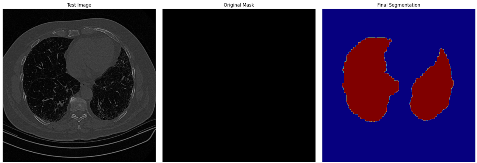
Final segmentation image on test data 

Conclusion

Fine-tuning SAM2 offers a practical way to enhance its capabilities for specific tasks. Whether you’re working on medical imaging, autonomous vehicles, or video editing, fine-tuning allows you to use SAM2 for your unique needs. By following this guide, you can adapt SAM2 for your projects and achieve state-of-the-art segmentation results.

For more advanced use cases, consider fine-tuning additional components of SAM2, such as the image encoder. While this requires more resources, it offers greater flexibility and performance improvements.