TensorBoard 教程：运行示例与使用 Logdir

本教程将指导您如何使用 TensorBoard，这是一款可以可视化数据及其行为的出色工具。您将了解在训练神经网络时，它可以用于哪些目的。

首先，您将学习如何启动 TensorBoard，随后了解其提供的不同视图。
接着，您将看到如何可视化计算过程中产生的标量值。您还将学习如何从模型中获取洞察，以修复学习中的潜在错误。
随后，您将探索如何将向量或数据集合以直方图的形式可视化。
借助该视图，您将比较神经网络的权重初始化如何影响学习过程中神经网络的权重更新。

提示：在此处查看 DataCamp 使用 Keras 的深度学习课程。

在开始之前，请确保导入以下库以成功运行代码：

from pandas_datareader import data
import matplotlib.pyplot as plt
import pandas as pd
import datetime as dt
import urllib.request, json
import os
import numpy as np

# This code has been tested with TensorFlow 1.6
import tensorflow as tf
from tensorflow.examples.tutorials.mnist import input_data
技术支持

启动 TensorBoard

要通过 TensorBoard 可视化内容，您首先需要启动其服务。为此，

打开命令提示符（Windows）或终端（Ubuntu/Mac）
进入项目主目录
如果您使用 Python virtualenv，请激活安装了 TensorFlow 的虚拟环境
确保可以通过 Python 看到 TensorFlow 库。为此，
- 输入 python3，您将看到类似 >>> 的提示符
- 尝试 import tensorflow as tf
- 如果能成功运行，说明没问题
通过输入 exit() 退出 Python 提示符（即 >>>），然后输入以下命令
- tensorboard --logdir=summaries
- --logdir 是您将创建用于可视化数据的目录
- TensorBoard 保存数据的文件称为事件文件
- 保存到事件文件中的数据类型称为摘要数据
- 可选地，您可以使用 --port=<port_you_like> 更改 TensorBoard 运行的端口
您现在应会看到如下信息
- TensorBoard 1.6.0 at <url>:6006 (Press CTRL+C to quit)
在浏览器中输入 <url>:6006
- 此时您应能看到一个橙色的仪表盘。由于尚未生成数据，因此不会有可显示的内容。

注意：TensorBoard 不喜欢在同一目录下看到多个事件文件。这可能导致显示出非常难看的曲线。因此，您应为每个不同示例创建单独的文件夹（例如，summaries/first、summaries/second、…）来保存数据。另一个需要注意的是，如果您要重新运行某个实验（即将事件文件保存到已存在文件的文件夹），必须先删除现有的事件文件。

TensorBoard 的不同视图

不同视图接收不同格式的输入并以不同方式显示。您可以在顶部橙色栏中切换。

Scalars（标量）- 可视化标量值，例如分类准确率。
Graph（图）- 可视化模型的计算图，例如神经网络模型。
Distributions（分布）- 可视化数据随时间的变化，例如神经网络的权重。
Histograms（直方图）- 更炫的分布视图，以三维的方式展示分布
Projector（投影）- 可用于可视化词嵌入（即词嵌入是对词的数值表示，能捕捉其语义关系）
Image（图像）- 可视化图像数据
Audio（音频）- 可视化音频数据
Text（文本）- 可视化文本（字符串）数据

在本教程中，您将涵盖加粗显示的视图。

理解标量可视化的益处

在本节中，您将首先了解为什么可视化某些指标（例如损失或准确率）是有益的。在训练深度神经网络时，初学者面临的关键问题之一，是缺乏对各种设计选择和超参数影响的理解。

例如，如果不加选择地将深度神经网络的权重初始化为方差很大的值，模型会很快发散并崩溃。另一方面，即使您相当擅长驯服神经网络加以利用，事情仍可能出错。例如，不关注学习率可能导致模型发散，或过早饱和于次优性能。

快速发现模型问题的一种方法，是实时（例如每 100 次迭代）以图形化方式观察模型内部发生的情况。这样一来，如果模型行为异常，将会一目了然。这正是 TensorBoard 为您提供的功能。您可以决定需要显示哪些值，TensorBoard 会在学习过程中对这些值进行实时可视化。

您将从创建一个用于手写数字分类的五层神经网络开始。为此，您将使用著名的 MNIST 数据集。TensorFlow 提供了简洁的 API 来加载 MNIST 数据，您无需手动下载。在此之前，您先定义一个简单的方法（即 accuracy()），用于计算某些预测相对于真实标签的准确率。

def accuracy(predictions,labels):
    '''
    Accuracy of a given set of predictions of size (N x n_classes) and
    labels of size (N x n_classes)
    '''
    return np.sum(np.argmax(predictions,axis=1)==np.argmax(labels,axis=1))*100.0/labels.shape[0]
技术支持

定义输入、输出、权重和偏置

首先，定义 batch_size，表示在一次优化/验证或测试步骤中采样的数据量。然后定义 layer_ids，为将要定义的神经网络各层提供标识。接着可以定义 layer_sizes。

请注意，len(layer_sizes) 应为 len(layer_ids)+1，因为 layer_sizes 包含最开始的输入大小。

MNIST 的图像大小为 28x28，展开为一维后为 784。然后您可以定义稍后用于训练模型的输入和标签占位符。最后，为每一层定义两个 TensorFlow 变量（即 weights 和 bias）。

您可以使用变量作用域（更多信息见此处），以便变量命名清晰，后续更易访问。

batch_size = 100
layer_ids = ['hidden1','hidden2','hidden3','hidden4','hidden5','out']
layer_sizes = [784, 500, 400, 300, 200, 100, 10]

tf.reset_default_graph()

# Inputs and Labels
train_inputs = tf.placeholder(tf.float32, shape=[batch_size, layer_sizes[0]], name='train_inputs')
train_labels = tf.placeholder(tf.float32, shape=[batch_size, layer_sizes[-1]], name='train_labels')

# Weight and Bias definitions
for idx, lid in enumerate(layer_ids):

    with tf.variable_scope(lid):
        w = tf.get_variable('weights',shape=[layer_sizes[idx], layer_sizes[idx+1]],
                            initializer=tf.truncated_normal_initializer(stddev=0.05))
        b = tf.get_variable('bias',shape= [layer_sizes[idx+1]],
                            initializer=tf.random_uniform_initializer(-0.1,0.1))
技术支持

计算 Logits、预测、损失与优化

定义完输入/输出占位符以及各层的权重和偏置后，您现在可以定义计算过程来求取神经网络的 logits。Logits 是神经网络最后一层产生的未归一化值。归一化后，我们称其为预测。这涉及遍历神经网络的每一层并计算 tf.matmul(h,w) +b。除了最后一层外，您还需要对所有层应用激活函数，如 tf.nn.relu(tf.matmul(h,w) +b)。

接下来，定义用于优化神经网络的损失函数。在本示例中，您可以使用交叉熵损失，它在分类问题中通常比均方误差效果更好。

最后，您需要定义一个优化器，它接受损失并按最小化损失的方向更新神经网络的权重。

# Calculating Logits
h = train_inputs
for lid in layer_ids:
    with tf.variable_scope(lid,reuse=True):
        w, b = tf.get_variable('weights'), tf.get_variable('bias')
        if lid != 'out':
          h = tf.nn.relu(tf.matmul(h,w)+b,name=lid+'_output')
        else:
          h = tf.nn.xw_plus_b(h,w,b,name=lid+'_output')

tf_predictions = tf.nn.softmax(h, name='predictions')
# Calculating Loss
tf_loss = tf.reduce_mean(tf.nn.softmax_cross_entropy_with_logits_v2(labels=train_labels, logits=h),name='loss')

# Optimizer
tf_learning_rate = tf.placeholder(tf.float32, shape=None, name='learning_rate')
optimizer = tf.train.MomentumOptimizer(tf_learning_rate,momentum=0.9)
grads_and_vars = optimizer.compute_gradients(tf_loss)
tf_loss_minimize = optimizer.minimize(tf_loss)
技术支持

定义摘要

此处您可以定义 tf.summary 对象。这些对象是 TensorBoard 能理解的实体。这意味着，凡是您希望显示的值，都应封装为 tf.summary 对象。

摘要有多种类型。此处由于仅可视化标量，您可以定义 tf.summary.scalar 对象。此外，您可以使用 tf.name_scope 在面板上对标量分组。也就是说，具有相同名称作用域的标量会显示在同一行。此处您定义三个不同的摘要。

tf_loss_summary：每当需要将其发布到面板时，您通过占位符馈入一个值
tf_accuracy_summary：每当需要将其发布到面板时，您通过占位符馈入一个值
tf_gradnorm_summary：用于计算神经网络最后一层梯度的 l2 范数。梯度范数是判断神经网络权重是否被正确更新的良好指标。过小的梯度范数可能表明梯度消失，过大的梯度可能意味着梯度爆炸现象。

# Name scope allows you to group various summaries together
# Summaries having the same name_scope will be displayed on the same row
with tf.name_scope('performance'):
    # Summaries need to be displayed
    # Whenever you need to record the loss, feed the mean loss to this placeholder
    tf_loss_ph = tf.placeholder(tf.float32,shape=None,name='loss_summary')
    # Create a scalar summary object for the loss so it can be displayed
    tf_loss_summary = tf.summary.scalar('loss', tf_loss_ph)

    # Whenever you need to record the loss, feed the mean test accuracy to this placeholder
    tf_accuracy_ph = tf.placeholder(tf.float32,shape=None, name='accuracy_summary')
    # Create a scalar summary object for the accuracy so it can be displayed
    tf_accuracy_summary = tf.summary.scalar('accuracy', tf_accuracy_ph)

# Gradient norm summary
for g,v in grads_and_vars:
    if 'hidden5' in v.name and 'weights' in v.name:
        with tf.name_scope('gradients'):
            tf_last_grad_norm = tf.sqrt(tf.reduce_mean(g**2))
            tf_gradnorm_summary = tf.summary.scalar('grad_norm', tf_last_grad_norm)
            break
# Merge all summaries together
performance_summaries = tf.summary.merge([tf_loss_summary,tf_accuracy_summary])
技术支持

执行神经网络：加载数据、训练、验证与测试

在下面的代码中，您将执行以下操作。首先，创建一个会话，用于执行前面定义的操作。然后，创建一个用于保存摘要数据的文件夹。接着，创建摘要写入器 summ_writer。现在可以初始化所有变量。随后加载 MNIST 数据集。

然后，对于每个 epoch 以及训练数据中的每个批次（即每次迭代），如果是第一次迭代则执行 gradnorm_summary，并使用摘要写入器将 gradnorm_summary 写入事件文件。接下来执行模型优化和损失计算。在完成单个 epoch 的全部训练数据后，计算平均训练损失。

对验证数据集也进行类似处理。具体来说，对于验证数据中的每个批次，计算验证准确率。随后，计算完整验证集的平均验证准确率。

最后，执行测试阶段。在该阶段，对于测试数据中的每个批次，计算每个批次的测试准确率。随后计算完整测试集的平均测试准确率。最后执行 performance_summaries，并使用摘要写入器将其写入事件文件。


image_size = 28
n_channels = 1
n_classes = 10
n_train = 55000
n_valid = 5000
n_test = 10000
n_epochs = 25

config = tf.ConfigProto(allow_soft_placement=True)
config.gpu_options.allow_growth = True
config.gpu_options.per_process_gpu_memory_fraction = 0.9 # making sure Tensorflow doesn't overflow the GPU

session = tf.InteractiveSession(config=config)

if not os.path.exists('summaries'):
    os.mkdir('summaries')
if not os.path.exists(os.path.join('summaries','first')):
    os.mkdir(os.path.join('summaries','first'))

summ_writer = tf.summary.FileWriter(os.path.join('summaries','first'), session.graph)

tf.global_variables_initializer().run()

accuracy_per_epoch = []
mnist_data = input_data.read_data_sets('MNIST_data', one_hot=True)


for epoch in range(n_epochs):
    loss_per_epoch = []
    for i in range(n_train//batch_size):

        # =================================== Training for one step ========================================
        batch = mnist_data.train.next_batch(batch_size)    # Get one batch of training data
        if i == 0:
            # Only for the first epoch, get the summary data
            # Otherwise, it can clutter the visualization
            l,_,gn_summ = session.run([tf_loss,tf_loss_minimize,tf_gradnorm_summary],
                                      feed_dict={train_inputs: batch[0].reshape(batch_size,image_size*image_size),
                                                 train_labels: batch[1],
                                                tf_learning_rate: 0.0001})
            summ_writer.add_summary(gn_summ, epoch)
        else:
            # Optimize with training data
            l,_ = session.run([tf_loss,tf_loss_minimize],
                              feed_dict={train_inputs: batch[0].reshape(batch_size,image_size*image_size),
                                         train_labels: batch[1],
                                         tf_learning_rate: 0.0001})
        loss_per_epoch.append(l)

    print('Average loss in epoch %d: %.5f'%(epoch,np.mean(loss_per_epoch)))    
    avg_loss = np.mean(loss_per_epoch)

    # ====================== Calculate the Validation Accuracy ==========================
    valid_accuracy_per_epoch = []
    for i in range(n_valid//batch_size):
        valid_images,valid_labels = mnist_data.validation.next_batch(batch_size)
        valid_batch_predictions = session.run(
            tf_predictions,feed_dict={train_inputs: valid_images.reshape(batch_size,image_size*image_size)})
        valid_accuracy_per_epoch.append(accuracy(valid_batch_predictions,valid_labels))

    mean_v_acc = np.mean(valid_accuracy_per_epoch)
    print('\tAverage Valid Accuracy in epoch %d: %.5f'%(epoch,np.mean(valid_accuracy_per_epoch)))

    # ===================== Calculate the Test Accuracy ===============================
    accuracy_per_epoch = []
    for i in range(n_test//batch_size):
        test_images, test_labels = mnist_data.test.next_batch(batch_size)
        test_batch_predictions = session.run(
            tf_predictions,feed_dict={train_inputs: test_images.reshape(batch_size,image_size*image_size)}
        )
        accuracy_per_epoch.append(accuracy(test_batch_predictions,test_labels))

    print('\tAverage Test Accuracy in epoch %d: %.5f\n'%(epoch,np.mean(accuracy_per_epoch)))
    avg_test_accuracy = np.mean(accuracy_per_epoch)

    # Execute the summaries defined above
    summ = session.run(performance_summaries, feed_dict={tf_loss_ph:avg_loss, tf_accuracy_ph:avg_test_accuracy})

    # Write the obtained summaries to the file, so it can be displayed in the TensorBoard
    summ_writer.add_summary(summ, epoch)

session.close()
技术支持

Successfully downloaded train-images-idx3-ubyte.gz 9912422 bytes.
Extracting MNIST_data/train-images-idx3-ubyte.gz
Successfully downloaded train-labels-idx1-ubyte.gz 28881 bytes.
Extracting MNIST_data/train-labels-idx1-ubyte.gz
Successfully downloaded t10k-images-idx3-ubyte.gz 1648877 bytes.
Extracting MNIST_data/t10k-images-idx3-ubyte.gz
Successfully downloaded t10k-labels-idx1-ubyte.gz 4542 bytes.
Extracting MNIST_data/t10k-labels-idx1-ubyte.gz
Average loss in epoch 0: 2.30252
    Average Valid Accuracy in epoch 0: 10.02000
    Average Test Accuracy in epoch 0: 9.76000

Average loss in epoch 1: 2.30016
    Average Valid Accuracy in epoch 1: 12.56000
    Average Test Accuracy in epoch 1: 12.64000

  ...
  ...
  ...

Average loss in epoch 24: 1.03386
    Average Valid Accuracy in epoch 24: 71.88000
    Average Test Accuracy in epoch 24: 71.23000
技术支持

可视化计算图

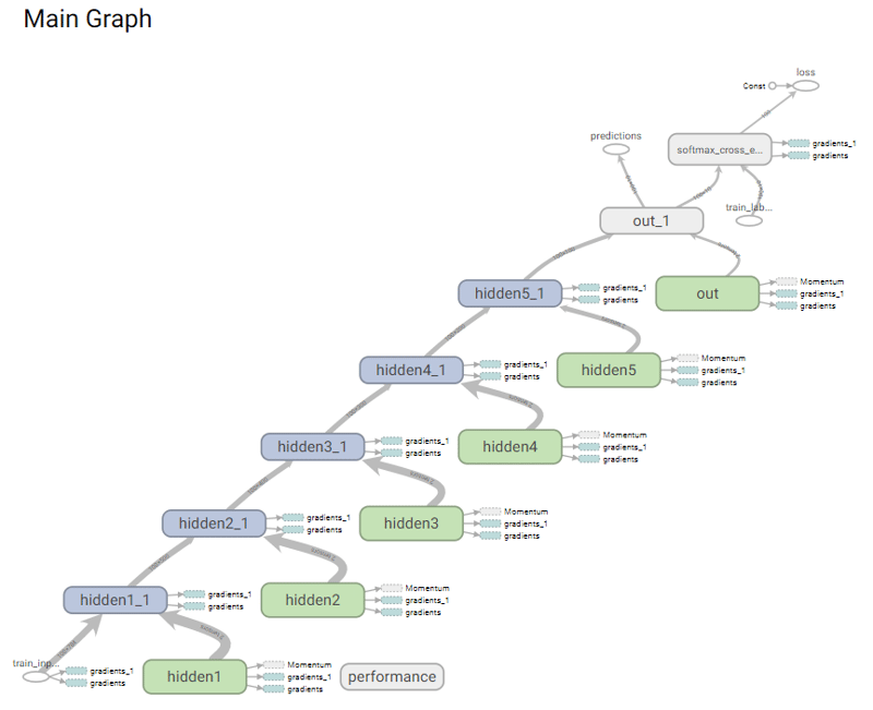
首先，您将看到模型的计算图长什么样。您可以点击 TensorBoard 中的Graphs 视图来访问该页面。它应当类似下图。您可以看到从 train_inputs 到 loss 和 predictions 通过隐藏层1 到 5 的清晰流向。

可视化摘要数据

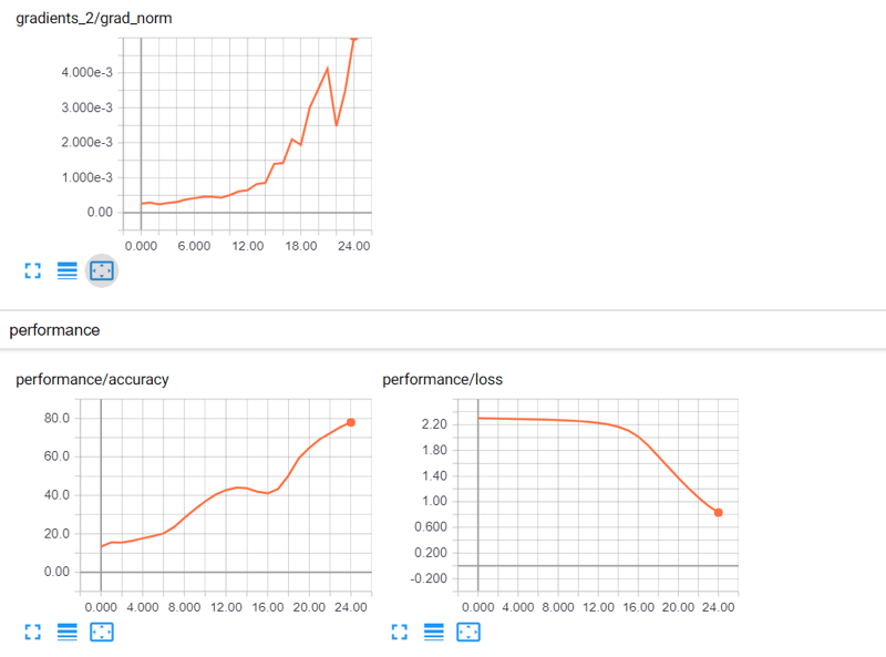
MNIST 分类是最简单的示例之一，但即便如此，使用 5 层神经网络仍未能解决。对于 MNIST，要在不到 5 个 epoch 内达到 90% 以上的准确率并不困难。

那么这里发生了什么？

让我们看一下 TensorBoard：

观察与结论

您可以看到准确率在上升，但非常缓慢，同时梯度更新随时间增加。这是种反常行为。如果正趋于收敛，您应看到梯度减小（接近零），而不是增大。但由于准确率在上升，说明方向是对的。您可能需要更高的学习率。

您现在可以尝试使用 0.01 的学习率。这与之前的神经网络执行几乎相同，只是将 0.0001 替换为 0.01。将 tf_learning_rate: 0.0001 改为 tf_learning_rate: 0.01。请注意有两个位置需要替换该参数。

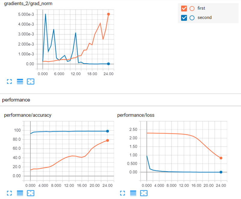
再看 TensorBoard：现在好得多

您现在会看到准确率一开始接近 100，且持续上升。同时，梯度更新也在随时间减小并趋近于零。使用 0.01 的学习率后情况好了很多。

接下来，让我们超越标量。您将看到如何分析标量向量和标量集合。

超越标量：可视化直方图/分布

您已经看到了通过 TensorBoard 可视化标量的好处，这使您能够了解模型的行为并修复模型的任何潜在问题。此外，可视化计算图还能让您看到从输入到预测之间存在不间断的连接，这对于梯度计算是必要的。

现在，您将看到 TensorBoard 中另一个有用的视图：直方图或分布。

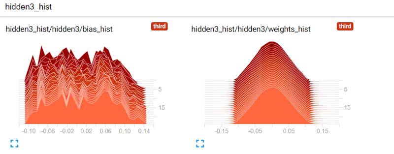
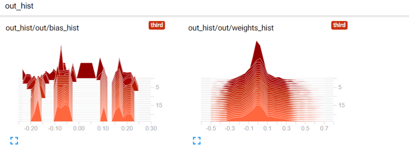
请记住，直方图是一组值，使用该值在集合中的频率/密度来表示。您可以使用直方图来可视化随时间变化的网络权重值。可视化网络权重很重要，因为如果权重在学习过程中大幅度跳动，这表明权重初始化或学习率存在问题。

您将在示例中看到权重如何变化。如果查看代码，会发现其使用 truncated_normal_initializer() 来初始化权重。

定义直方图摘要以可视化权重和偏置

此处您再次定义 tf.summary 对象。不过，现在您要可视化的是标量向量，因此需要定义 tf.summary.histogram 对象。

在这种情况下，您定义两个直方图对象（即 tf_w_hist 和 tf_b_hist），它们包含给定层的权重和偏置。您将为所有层定义此类直方图对象，每一层都有自己的名称作用域。

最后，您可以使用 tf.summary.merge 操作创建一个分组操作，一次性执行所有这些摘要。

# Summaries need to be displayed
# Create a summary for each weight bias in each layer
all_summaries = []
for lid in layer_ids:
    with tf.name_scope(lid+'_hist'):
        with tf.variable_scope(lid,reuse=True):
            w,b = tf.get_variable('weights'), tf.get_variable('bias')

            # Create a scalar summary object for the loss so it can be displayed
            tf_w_hist = tf.summary.histogram('weights_hist', tf.reshape(w,[-1]))
            tf_b_hist = tf.summary.histogram('bias_hist', b)
            all_summaries.extend([tf_w_hist, tf_b_hist])

# Merge all parameter histogram summaries together
tf_param_summaries = tf.summary.merge(all_summaries)
技术支持

执行神经网络（含直方图摘要）

此步骤与之前几乎相同，但这里您多了几行用于计算直方图摘要（即 tf_param_summaries）。

注意，学习率也再次发生了变化。

image_size = 28
n_channels = 1
n_classes = 10
n_train = 55000
n_valid = 5000
n_test = 10000
n_epochs = 25

config = tf.ConfigProto(allow_soft_placement=True)
config.gpu_options.allow_growth = True
config.gpu_options.per_process_gpu_memory_fraction = 0.9 # making sure Tensorflow doesn't overflow the GPU

session = tf.InteractiveSession(config=config)

if not os.path.exists('summaries'):
    os.mkdir('summaries')
if not os.path.exists(os.path.join('summaries','third')):
    os.mkdir(os.path.join('summaries','third'))

summ_writer_3 = tf.summary.FileWriter(os.path.join('summaries','third'), session.graph)

tf.global_variables_initializer().run()

accuracy_per_epoch = []
mnist_data = input_data.read_data_sets('MNIST_data', one_hot=True)


for epoch in range(n_epochs):
    loss_per_epoch = []
    for i in range(n_train//batch_size):

        # =================================== Training for one step ========================================
        batch = mnist_data.train.next_batch(batch_size)    # Get one batch of training data
        if i == 0:
            # Only for the first epoch, get the summary data
            # Otherwise, it can clutter the visualization
            l,_,gn_summ, wb_summ = session.run([tf_loss,tf_loss_minimize,tf_gradnorm_summary, tf_param_summaries],
                                      feed_dict={train_inputs: batch[0].reshape(batch_size,image_size*image_size),
                                                 train_labels: batch[1],
                                                tf_learning_rate: 0.00001})
            summ_writer_3.add_summary(gn_summ, epoch)
            summ_writer_3.add_summary(wb_summ, epoch)
        else:
            # Optimize with training data
            l,_ = session.run([tf_loss,tf_loss_minimize],
                              feed_dict={train_inputs: batch[0].reshape(batch_size,image_size*image_size),
                                         train_labels: batch[1],
                                         tf_learning_rate: 0.01})
        loss_per_epoch.append(l)

    print('Average loss in epoch %d: %.5f'%(epoch,np.mean(loss_per_epoch)))    
    avg_loss = np.mean(loss_per_epoch)

    # ====================== Calculate the Validation Accuracy ==========================
    valid_accuracy_per_epoch = []
    for i in range(n_valid//batch_size):
        valid_images,valid_labels = mnist_data.validation.next_batch(batch_size)
        valid_batch_predictions = session.run(
            tf_predictions,feed_dict={train_inputs: valid_images.reshape(batch_size,image_size*image_size)})
        valid_accuracy_per_epoch.append(accuracy(valid_batch_predictions,valid_labels))

    mean_v_acc = np.mean(valid_accuracy_per_epoch)
    print('\tAverage Valid Accuracy in epoch %d: %.5f'%(epoch,np.mean(valid_accuracy_per_epoch)))

    # ===================== Calculate the Test Accuracy ===============================
    accuracy_per_epoch = []
    for i in range(n_test//batch_size):
        test_images, test_labels = mnist_data.test.next_batch(batch_size)
        test_batch_predictions = session.run(
            tf_predictions,feed_dict={train_inputs: test_images.reshape(batch_size,image_size*image_size)}
        )
        accuracy_per_epoch.append(accuracy(test_batch_predictions,test_labels))

    print('\tAverage Test Accuracy in epoch %d: %.5f\n'%(epoch,np.mean(accuracy_per_epoch)))
    avg_test_accuracy = np.mean(accuracy_per_epoch)

    # Execute the summaries defined above
    summ = session.run(performance_summaries, feed_dict={tf_loss_ph:avg_loss, tf_accuracy_ph:avg_test_accuracy})

    # Write the obtained summaries to the file, so they can be displayed
    summ_writer_3.add_summary(summ, epoch)

session.close()
技术支持

Extracting MNIST_data/train-images-idx3-ubyte.gz
Extracting MNIST_data/train-labels-idx1-ubyte.gz
Extracting MNIST_data/t10k-images-idx3-ubyte.gz
Extracting MNIST_data/t10k-labels-idx1-ubyte.gz
Average loss in epoch 0: 1.02625
    Average Valid Accuracy in epoch 0: 92.76000
    Average Test Accuracy in epoch 0: 92.65000

Average loss in epoch 1: 0.19110
    Average Valid Accuracy in epoch 1: 95.80000
    Average Test Accuracy in epoch 1: 95.48000

  ...
  ...
  ...

Average loss in epoch 24: 0.00009
    Average Valid Accuracy in epoch 24: 98.28000
    Average Test Accuracy in epoch 24: 98.09000
技术支持

可视化权重和偏置的直方图数据

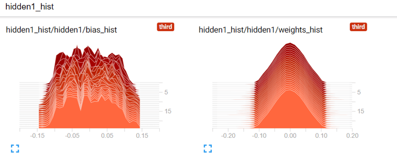
以下是您的权重和偏置的可视化。首先，您有三条坐标轴：时间（x 轴）、值（y 轴）以及数值的频率/密度（z 轴）。颜色更深的直方图代表更旧的数据，颜色更浅的代表更新的数据。z 轴数值越高，表示向量中越多的值接近该特定取值。

注意：您还可以查看直方图随时间的“叠加”视图。您可以在左侧选项面板中更改显示类型。

不同初始化器的影响

现在，您将不再使用 truncated_normal_initializer()，而使用 xavier_initializer() 来初始化权重。Xavier 初始化是一种更适合深度神经网络的初始化技术。

这是因为，与使用用户自定义标准差（使用 truncated_normal_initializer() 时的做法）不同，Xavier 初始化会根据某一层的输入和输出连接数自动决定标准差。这有助于让梯度从顶层到底层顺畅传播，避免出现如梯度消失的问题。然后您再次定义模型。

首先，定义 batch_size，表示一次优化/验证或测试步骤中采样的数据量。然后定义 layer_ids，为您将要定义的神经网络各层提供标识。

接着可以定义 layer_sizes。请注意，len(layer_sizes) 应为 len(layer_ids)+1，因为 layer_sizes 包含最开始的输入大小。MNIST 的图像大小为 28x28，展开为一维后为 784。

随后，您可以定义输入和标签占位符，稍后将用于训练模型。最后，为每一层定义两个 TensorFlow 变量（即 weights 和 bias）。

注意：这与您第一次使用的代码相同，唯一区别在于权重所用的初始化技术

batch_size = 100
layer_ids = ['hidden1','hidden2','hidden3','hidden4','hidden5','out']
layer_sizes = [784, 500, 400, 300, 200, 100, 10]

tf.reset_default_graph()

# Inputs and Labels
train_inputs = tf.placeholder(tf.float32, shape=[batch_size, layer_sizes[0]], name='train_inputs')
train_labels = tf.placeholder(tf.float32, shape=[batch_size, layer_sizes[-1]], name='train_labels')

# Weight and Bias definitions
for idx, lid in enumerate(layer_ids):

    with tf.variable_scope(lid):
        w = tf.get_variable('weights',shape=[layer_sizes[idx], layer_sizes[idx+1]],
                            initializer=tf.contrib.layers.xavier_initializer())
        b = tf.get_variable('bias',shape= [layer_sizes[idx+1]],
                            initializer=tf.random_uniform_initializer(-0.1,0.1))
技术支持

计算 Logits、预测、损失与优化

定义完输入/输出占位符以及各层的权重和偏置后，您现在可以再次定义计算过程来求取神经网络的 logits。

注意：此部分与您首次定义这些操作和张量时使用的代码完全相同。

定义摘要

此处您可以再次定义 tf.summary 对象。这也与您首次定义这些操作和张量时使用的代码相同。

直方图摘要：可视化权重和偏置

此处您再次定义 tf.summary 对象。不过，现在您要可视化的是标量向量，因此需要定义 tf.summary.histogram 对象。

注意，这与您首次定义这些操作和张量时使用的代码相同。

执行神经网络

注意，这与上一节中您所做的相同！

您只需更改少量代码：将三处 os.path.join('summaries','third') 改为 os.path.join('summaries','fourth')，将 summ_writer_3 改为 summ_writer_4（出现 4 次），并将 tf_learning_rate 的 0.00001 设置为 0.01。


image_size = 28
n_channels = 1
n_classes = 10
n_train = 55000
n_valid = 5000
n_test = 10000
n_epochs = 25

config = tf.ConfigProto(allow_soft_placement=True)
config.gpu_options.allow_growth = True
config.gpu_options.per_process_gpu_memory_fraction = 0.9 # making sure TensorFlow doesn't overflow the GPU

session = tf.InteractiveSession(config=config)

if not os.path.exists('summaries'):
    os.mkdir('summaries')
if not os.path.exists(os.path.join('summaries','fourth')):
    os.mkdir(os.path.join('summaries','fourth'))

summ_writer_4 = tf.summary.FileWriter(os.path.join('summaries','fourth'), session.graph)

tf.global_variables_initializer().run()

accuracy_per_epoch = []
mnist_data = input_data.read_data_sets('MNIST_data', one_hot=True)


for epoch in range(n_epochs):
    loss_per_epoch = []
    for i in range(n_train//batch_size):

        # =================================== Training for one step ========================================
        batch = mnist_data.train.next_batch(batch_size)    # Get one batch of training data
        if i == 0:
            # Only for the first epoch, get the summary data
            # Otherwise, it can clutter the visualization
            l,_,gn_summ, wb_summ = session.run([tf_loss,tf_loss_minimize,tf_gradnorm_summary, tf_param_summaries],
                                      feed_dict={train_inputs: batch[0].reshape(batch_size,image_size*image_size),
                                                 train_labels: batch[1],
                                                tf_learning_rate: 0.01})
            summ_writer_4.add_summary(gn_summ, epoch)
            summ_writer_4.add_summary(wb_summ, epoch)
        else:
            # Optimize with training data
            l,_ = session.run([tf_loss,tf_loss_minimize],
                              feed_dict={train_inputs: batch[0].reshape(batch_size,image_size*image_size),
                                         train_labels: batch[1],
                                         tf_learning_rate: 0.01})
        loss_per_epoch.append(l)

    print('Average loss in epoch %d: %.5f'%(epoch,np.mean(loss_per_epoch)))    
    avg_loss = np.mean(loss_per_epoch)

    # ====================== Calculate the Validation Accuracy ==========================
    valid_accuracy_per_epoch = []
    for i in range(n_valid//batch_size):
        valid_images,valid_labels = mnist_data.validation.next_batch(batch_size)
        valid_batch_predictions = session.run(
            tf_predictions,feed_dict={train_inputs: valid_images.reshape(batch_size,image_size*image_size)})
        valid_accuracy_per_epoch.append(accuracy(valid_batch_predictions,valid_labels))

    mean_v_acc = np.mean(valid_accuracy_per_epoch)
    print('\tAverage Valid Accuracy in epoch %d: %.5f'%(epoch,np.mean(valid_accuracy_per_epoch)))

    # ===================== Calculate the Test Accuracy ===============================
    accuracy_per_epoch = []
    for i in range(n_test//batch_size):
        test_images, test_labels = mnist_data.test.next_batch(batch_size)
        test_batch_predictions = session.run(
            tf_predictions,feed_dict={train_inputs: test_images.reshape(batch_size,image_size*image_size)}
        )
        accuracy_per_epoch.append(accuracy(test_batch_predictions,test_labels))

    print('\tAverage Test Accuracy in epoch %d: %.5f\n'%(epoch,np.mean(accuracy_per_epoch)))
    avg_test_accuracy = np.mean(accuracy_per_epoch)

    # Execute the summaries defined above
    summ = session.run(performance_summaries, feed_dict={tf_loss_ph:avg_loss, tf_accuracy_ph:avg_test_accuracy})

    # Write the obtained summaries to the file, so they can be displayed
    summ_writer_4.add_summary(summ, epoch)

session.close()
技术支持

Extracting MNIST_data/train-images-idx3-ubyte.gz
Extracting MNIST_data/train-labels-idx1-ubyte.gz
Extracting MNIST_data/t10k-images-idx3-ubyte.gz
Extracting MNIST_data/t10k-labels-idx1-ubyte.gz
Average loss in epoch 0: 0.43618
    Average Valid Accuracy in epoch 0: 95.70000
    Average Test Accuracy in epoch 0: 95.22000

Average loss in epoch 1: 0.12872
    Average Valid Accuracy in epoch 1: 96.86000
    Average Test Accuracy in epoch 1: 96.71000

  ...
  ...
  ...

Average loss in epoch 24: 0.00009
    Average Valid Accuracy in epoch 24: 98.42000
    Average Test Accuracy in epoch 24: 98.21000
技术支持

如何比较不同的初始化技术

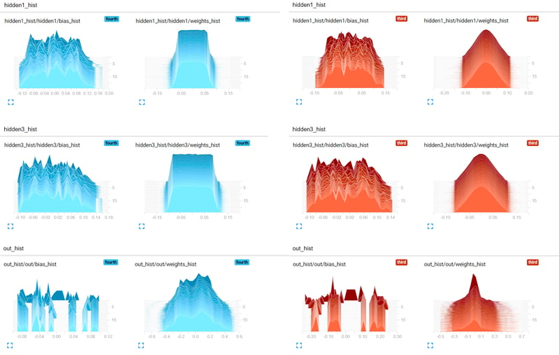
此处您可以比较两种不同初始化方式下权重随时间的演化：truncated_normal_initializer（红色）与 xavier_initializer（蓝色）。您可以看到，xavier_initializer 让更多权重远离零点，而非普通初始化器，这样做更好。这可能使得采用 Xavier 初始化的神经网络收敛更快，正如损失/准确率曲线所显示的那样。

直方图的分布视图

现在您可以比较两种视图的差异：直方图视图和分布视图。分布视图本质上是观察直方图的另一种方式。如果您查看下图，会很容易发现分布视图就是直方图视图的顶视图。请注意，在此情况下对直方图图像进行了旋转，便于更清晰地看到相似之处。

结论

在本教程中，您学习了如何使用 TensorBoard。首先，您了解了如何通过命令提示符（Windows）或终端（Ubuntu/Mac）启动其服务。接着，您查看了 TensorBoard 提供的不同数据视图。然后，您阅读了可视化标量值（例如损失/准确率）的代码，并使用前馈神经网络模型具体理解了标量可视化的用法。

随后，您探索了如何使用直方图视图可视化标量集合/向量。接着，通过直方图视图比较了神经网络权重初始化技术之间的差异。

最后，您讨论了分布视图与直方图视图之间的相似之处。

如果您想进一步学习深度学习，欢迎查看我们的Keras 深度学习课程。

查看我们的机器学习模型中的超参数优化教程，进一步了解参数与超参数。

如果您希望联系我，可以发邮件至 [email protected]，或通过LinkedIn 与我建立联系。

主题

人工智能机器学习深度学习

主题

技术

TensorBoard 教程

使用 AI 探索

启动 TensorBoard

TensorBoard 的不同视图

理解标量可视化的益处

定义输入、输出、权重和偏置

计算 Logits、预测、损失与优化

定义摘要

执行神经网络：加载数据、训练、验证与测试

可视化计算图

可视化摘要数据

观察与结论

再看 TensorBoard：现在好得多

超越标量：可视化直方图/分布

定义直方图摘要以可视化权重和偏置

执行神经网络（含直方图摘要）

可视化权重和偏置的直方图数据

不同初始化器的影响

计算 Logits、预测、损失与优化

定义摘要

直方图摘要：可视化权重和偏置

执行神经网络

如何比较不同的初始化技术

直方图的分布视图

结论

主题

进一步学习机器学习与深度学习

理解机器学习

Python 树模型机器学习

Python 深度学习入门

主题

技术

进一步学习机器学习与深度学习

理解机器学习

Python 树模型机器学习

Python 深度学习入门