使用 TimeGPT 进行时间序列预测

开始使用 TimeGPT

TimeGPT 模型不是开源的，您只能通过 Nixtla API 进行访问。本节将指导您配置 Nixtla API 来访问 TimeGPT 模型，并对亚马逊股票数据进行预测。

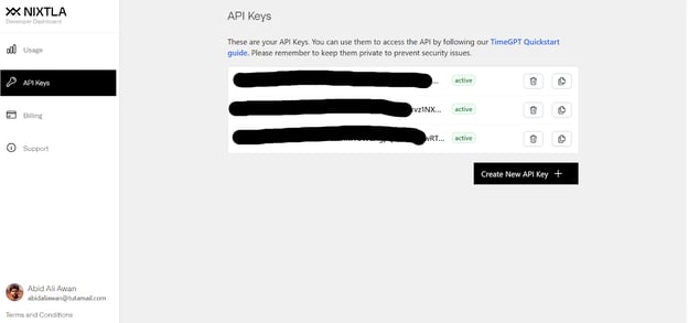
1. 我们需要访问 dashboard.nixtla.io 生成一个 API 密钥。系统会提示我们创建账户以生成 API 密钥。目前可以免费访问 TimeGPT，但对 API 调用次数有一定限制。

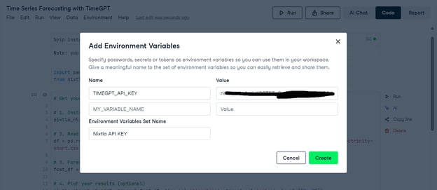
2. 我们使用 DataCamp 的DataLab 作为编码环境。DataLab 是免费的云端 Jupyter Notebook，任何人都能在几秒内开始编码。要在 DataLab 中设置环境变量，点击 "Environment" 选项卡，然后点击 "Environment variables..." 按钮，接着点击 "+ Add"，添加变量名和 API 密钥。

3. 安装用于该模型的 Nixtla Python 客户端，以及用于股票数据集的 Yahoo Finance 库。 

%%capture
%pip install nixtla>=0.5.1
%pip install yfinance技术支持

4. 使用 TimeGPT 的 API 密钥创建 Nixtla 客户端。
5. 下载亚马逊股价数据，重置索引，并展示前五行。

import pandas as pd
import yfinance as yf
from nixtla import NixtlaClient
import os

timegpt_api_key = os.environ["TIMEGPT_API_KEY"]

# Setup NixtlaClient
nixtla_client = NixtlaClient(api_key = timegpt_api_key)


# Downloading Amazon stock price data
ticker = 'AMZN'
amazon_stock_data = yf.download(ticker)
amazon_stock_data = amazon_stock_data.reset_index()

# Displaying the dataset
amazon_stock_data.head()技术支持

我们拥有自 1997 年起至今的亚马逊股价数据。

6. 我们可以直接使用 Nixtla 客户端绘制股价数据。 

nixtla_client.plot(amazon_stock_data, time_col='Date', target_col='Close')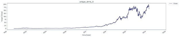技术支持

想要了解如何使用 Matplotlib 创建时间序列折线图，请参阅本Matplotlib 时间序列折线图教程。

7. 要进行预测，我们需要为 .forecast 函数提供股价数据、模型名称、预测视窗（相当于 24 天）、频率、时间列与目标列。由于证券交易所周末休市，我们将频率设为“工作日(B)”。

model = nixtla_client.forecast(
    df=amazon_stock_data,
    model="timegpt-1",
    h=24,
    freq="B",
    time_col="Date",
    target_col="Close",
)
model.tail()
技术支持

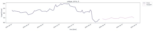
8. 使用最大样本长度 60 绘制真实与预测数据集。这意味着仅绘制最近的 60 个值，以更聚焦地展示模型预测。

nixtla_client.plot(
    amazon_stock_data,
    model,
    time_col="Date",
    target_col="Close",
    max_insample_length=60,
)
技术支持

可以看到，短短几秒内，TimeGPT 模型就准确预测了亚马逊的未来收盘价。 

以上是入门示例。接下来，我们将处理更复杂的数据集，并探索 Nixtla API 的更多功能。

使用 TimeGPT 预测澳大利亚用电需求

本节我们将使用更复杂的澳大利亚用电需求数据集，使用 TimeGPT 模型一次性预测多个值。 

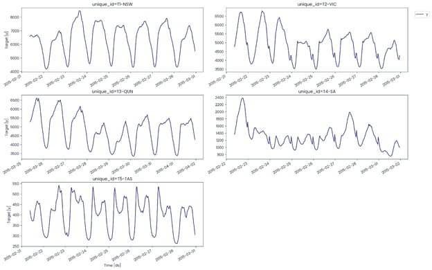
该数据集包含 5 条时间序列，表示澳大利亚 5 个州（维多利亚州、新南威尔士州、昆士兰州、塔斯马尼亚州和南澳大利亚州）的半小时用电需求。

我们还将学习如何对模型进行微调，并使用多种超参数来提升性能。最后，我们将进行交叉验证，并与传统模型对比，完成更全面的评估。

加载数据集

pandas 库并没有简单的方法来加载 .tsf 文件。我们需要自定义函数来加载和处理数据，然后将其转换为 Pandas 数据框。

import pandas as pd


def read_tsf_from_file(file_path):
    data = []
    start_date = pd.to_datetime("2002-01-01 00:00:00")

    # Open and read the file from the directory

    with open(file_path, "r") as file:
        for line in file:
            if line.startswith("T"):
                parts = line.strip().split(":")
                unique_id = parts[0] + "-" + parts[1]
                values = list(map(float, parts[3].split(",")[:-1]))

                # Generate datetime index at half-hour intervals

                periods = len(values)
                date_range = pd.date_range(
                    start=start_date, periods=periods, freq="30min"
                )

                # Append to data list

                for dt, value in zip(date_range, values):
                    data.append([unique_id, dt, value])
    # Convert the list of data into a DataFrame

    return pd.DataFrame(data, columns=["unique_id", "ds", "y"])


# Example usage

file_path = "australian_electricity_demand_dataset.tsf"
demand_df = read_tsf_from_file(file_path)

# Display the dataframe

demand_df.head()
技术支持

数据集包含三列： 

1. unique_id：代表澳大利亚的 5 个州。
2. ds：日期与时间。
3. y：用电需求。

plot 函数非常好用，它会自动识别 unique_id 列，并创建五个不同的时间序列可视化。

nixtla_client.plot(
    demand_df, 
    max_insample_length=365, 
)技术支持

下方可视化展示了 5 个州的用电量，它们的模式并不相同。

通过参加DataCamp 的直播代码实操，学习时间序列分析，使用 Python 深入金融时间序列数据集。 

在本次课程中，我们将探索多只股票、可视化其表现，并使用不同模型进行预测。

异常检测

在预测之前，我们先识别数据集中的各种异常，以便更好地理解问题。 

.detect_anomalies 函数接收数据集、时间列、目标列和频率作为参数。 

# Detect anomalies
anomalies_df = nixtla_client.detect_anomalies(
    demand_df, 
    time_col='ds', 
    target_col='y', 
    freq='H', 
)
anomalies_df[anomalies_df["anomaly"]==1].head()技术支持

上方展示的是检测到异常的实例。 

5 条时间序列中异常的总数为 17,316，数量相当多。

anomalies_df.anomaly.value_counts()技术支持

现在，我们将在真实数据上绘制异常，以查看它们出现的位置和日常频率。为简化可视化，我们仅展示新南威尔士州的 5,000 个样本。

# Plot anomalies
nixtla_client.plot(
    demand_df[demand_df["unique_id"]=="T1-NSW"][0:5000], 
    anomalies_df[anomalies_df["unique_id"]=="T1-NSW"][0:5000],
    time_col='ds', 
    target_col='y',
    
)技术支持

从日度来看，异常并不常见，但确实存在某些天内多次异常的情况。

使用 TimeGPT 的单序列预测

现在我们来预测新南威尔士州的用电需求。为此，将仅筛选出 “T1-NSW” 的数值。

T1_df = demand_df[demand_df["unique_id"]=="T1-NSW"]
T1_df.head()技术支持

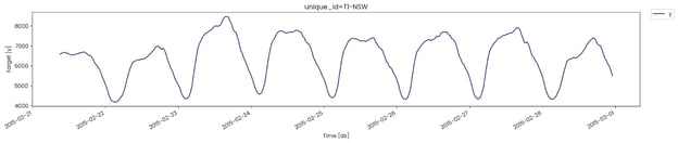
绘制最近 365 个值，以了解用电模式。 

nixtla_client.plot(
    T1_df, 
    max_insample_length=365, 
)技术支持

接下来评估模型表现。为此，我们需要将数据集划分为训练集和测试集。 

训练集包含 144 个值（相当于 3 天），测试集包含 1200 个值（相当于 25 天）。

test_df = T1_df.tail(144) # 3 days = (144 * 0.5h *  1 day/24h) 
train_df = T1_df.iloc[-1344:-144] # 25 days = (1200 *0.5h * 1 day/24h)技术支持

在预测时，我们将选择更合适的模型，并设置多个参数以提升表现，具体包括：

1. 预测接下来的 144 个值（3 天）。
2. 预测 90% 置信区间。 
3. 以 60 个步骤微调模型，虽然步数较多，但能带来更好结果。 
4. 将损失函数设为 MAE。 
5. 使用 TimeGPT-1-long-horizon 模型替代简单模型。 
6. 设置时间列与目标列。 

predict_df = nixtla_client.forecast(
    df=train_df,
    h=144,
    level=[90],  # Generate a 90% confidence interval
    finetune_steps=60,  # Specify the number of steps for fine-tuning
    finetune_loss="mae",  # Use the MAE as the loss function for fine-tuning
    model="timegpt-1-long-horizon",  # Use the model for long-horizon forecasting
    time_col="ds",
    target_col="y",
)
技术支持

绘制真实值、预测值与 90% 置信区间，以评估模型表现。

nixtla_client.plot(
    test_df, predict_df, models=["TimeGPT"], level=[90], time_col="ds", target_col="y"
)
技术支持

短短几秒即可得到相当准确的结果——这正是预训练模型的强大之处。

接下来，我们将使用 Nixtla 开源项目中的 UtilsForecast 库评估模型表现。我们会先合并测试集与预测集，然后将其传入 evaluate 函数。该函数接收数据集、指标、模型、目标列与唯一 ID，用于计算模型指标，并以 pandas 数据框形式展示。

from utilsforecast.losses import mae, rmse, smape
from utilsforecast.evaluation import evaluate

predict_df["ds"] = pd.to_datetime(predict_df["ds"])
test_df = pd.merge(test_df, predict_df, "left", ["ds", "unique_id"])
evaluation = evaluate(
    test_df,
    metrics=[mae, rmse, smape],
    models=["TimeGPT"],
    target_col="y",
    id_col="unique_id",
)

average_metrics = evaluation.groupby("metric")["TimeGPT"].mean()
average_metrics技术支持

我们得到了相当不错的结果。 

使用 TimeGPT 的多序列预测

Nixtla API 也支持一次性预测多条序列。我们将使用整个数据集，而非按唯一 ID 进行筛选。 

为了划分训练集和测试集，我们使用 groupby 函数为每个唯一 ID 切分出 144 个值。否则，我们可能只会得到某个随机唯一 ID 的 144 个值。

values for some randomly chosen unique ID.
test_df = demand_df.groupby("unique_id").tail(144)  # 3 days
train_df = (
    demand_df.groupby("unique_id")
    .apply(lambda group: group.iloc[-1344:-144])
    .reset_index(drop=True)
)  # 25 days技术支持

forecast 函数与前一部分相同，但这次我们还包含了 ID 列。

predict_df = nixtla_client.forecast(
    df=train_df,
    h=144,                            
    level=[90],                        
    finetune_steps=60,                 
    finetune_loss='mae',               
    model='timegpt-1-long-horizon',    
    time_col='ds',
    target_col='y',
    id_col='unique_id'
)技术支持

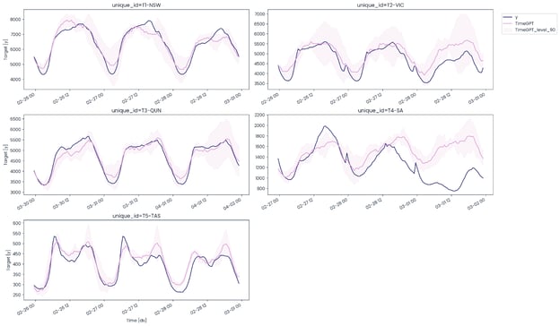
为所有 5 个唯一 ID 绘制真实值、预测值与 90 置信水平的时间序列图。

nixtla_client.plot(
    test_df, predict_df, models=["TimeGPT"], level=[90], time_col="ds", target_col="y"
)技术支持

可以看到，TimeGPT 模型在多条时间序列上的表现仍然不错，除了南澳大利亚州。它未能预测出用电需求的下降趋势。

为使用 MAE、RMSE 与 SMAPE 指标评估模型，我们需要合并测试与预测数据框。

predict_df['ds'] = pd.to_datetime(predict_df['ds'])
test_df = pd.merge(test_df, predict_df, 'left', ['ds','unique_id'])技术支持

使用 evaluate 函数生成模型表现报告（pandas 数据框）。其中将包含每个唯一 ID 的模型指标。要计算模型的整体表现，我们需要对这些值取平均并展示最终结果。 

evaluation = evaluate(
    test_df,
    metrics=[mae, rmse, smape],
    models=["TimeGPT"],
    target_col="y",
    id_col = "unique_id"
)

average_metrics = evaluation.groupby('metric')["TimeGPT"].mean()
average_metrics技术支持

与单一序列微调相比，在多条时间序列上微调能够整体提升模型表现。

交叉验证

Nixtla 客户端还支持对数据集的多个窗口执行交叉验证，以评估模型表现。

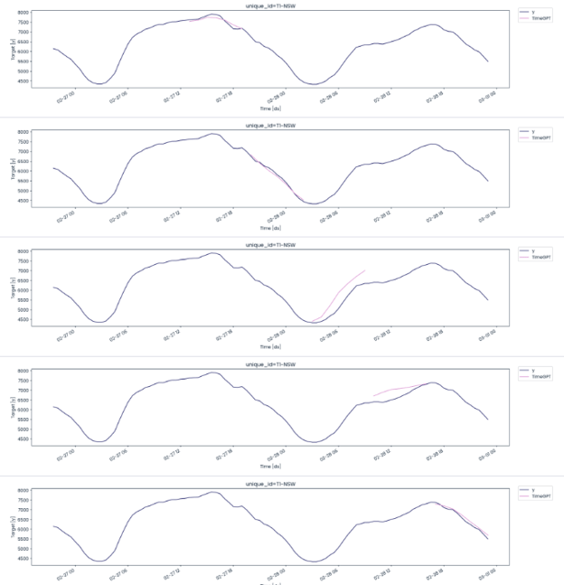
我们将使用 .cross_validation 函数，并传入仅包含新南威尔士州数据的筛选数据集。交叉验证将包含 5 个窗口，每个窗口长度为 7 小时。

timegpt_cv_df = nixtla_client.cross_validation(
    T1_df, 
    h=7, 
    n_windows=5, 
    time_col='ds', 
    target_col='y', 
    freq='H',
)
timegpt_cv_df.head()技术支持

可以看到，我们基于五个 7 小时的窗口获得了预测值。

我们将使用截断日期时间来创建 5 个窗口，分别展示预测值与真实值。

cutoffs = timegpt_cv_df['cutoff'].unique()
for cutoff in cutoffs:
    fig = nixtla_client.plot(
        T1_df.tail(100), 
        timegpt_cv_df.query('cutoff == @cutoff').drop(columns=['cutoff', 'y']),
        time_col='ds', 
        target_col='y'
    )
    display(fig)技术支持

除第 3 与第 4 次划分外，模型整体表现相当不错。

LGBM 与 TimeGPT 的对比

现在我们将比较 TimeGPT 与 Light Gradient-Boosting Machine（LGBM）模型的表现，以明确哪一个在同一数据集上更胜一筹。我们已对新南威尔士州的数据框进行了交叉验证；下一步是使用 evaluate 函数生成模型评估报告。

evaluation = evaluate(
    timegpt_cv_df,
    metrics=[mae, rmse, smape],
    models=["TimeGPT"],
    target_col="y",
    id_col = "cutoff"
)
evaluation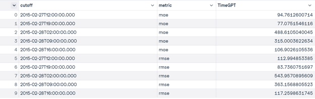技术支持

我们需要对 5 个窗口的 MAE、RMSE 与 SMAPE 取均值，以获得模型的整体结果。

average_metrics = evaluation.groupby('metric')["TimeGPT"].mean()
average_metrics技术支持

即便在较小的数据量上，结果也相当不错。 

评估 LGBM 模型需要遵循以下步骤：

1. 数据筛选： 确保数据与 TimeGPT 交叉验证所用值一致或相近。
2. 日期时间转换： 将日期时间信息转换为数值。
3. 特征工程： 使用滞后与滚动窗口技巧创建额外特征。
4. 缺失值处理： 删除因创建滞后与滚动窗口而产生的缺失值。
5. 建模准备： 定义特征矩阵 X 与目标向量 y，并使用 TimeSeriesSplit 划分。
6. 训练与评估： 训练模型、进行评估，并记录每个数据划分的指标。
7. 结果汇总： 计算各项模型指标的均值，并以 pandas 数据框展示。

注意：若要使用统计与机器学习模型进行时间序列预测，掌握基础的特征工程技巧与算法至关重要。详尽指南请参阅本教程：DataCamp 上的时间序列预测教程。

import pandas as pd
import numpy as np
import lightgbm as lgb
from sklearn.model_selection import TimeSeriesSplit
from sklearn.metrics import mean_absolute_error, mean_squared_error

# Function to calculate SMAPE
def smape(y_true, y_pred):
    return np.mean(2 * np.abs(y_pred - y_true) / (np.abs(y_true) + np.abs(y_pred)))

# Assuming 'ds' is the date/time column and 'y' is the target variable
T1_df['ds'] = pd.to_datetime(T1_df['ds'])

# Filter the DataFrame to include only the specified datetime range
start_date = '2015-02-27T13:00:00'
end_date = '2015-02-28T23:00:00'
T1_df = T1_df[(T1_df['ds'] >= start_date) & (T1_df['ds'] <= end_date)]

# Convert 'ds' to a numerical value (e.g., timestamp)
T1_df['ds_num'] = T1_df['ds'].apply(lambda x: x.timestamp())

# Create lag and window features
for lag in range(1, 4):
    T1_df[f'lag_{lag}'] = T1_df['y'].shift(lag)

T1_df['rolling_mean'] = T1_df['y'].rolling(window=3).mean()
T1_df['rolling_std'] = T1_df['y'].rolling(window=3).std()

# Drop NaN values resulting from lag and rolling operations
T1_df.dropna(inplace=True)

# Select features for the model
X = T1_df[['ds_num', 'lag_1', 'lag_2', 'lag_3', 'rolling_mean', 'rolling_std']]
y = T1_df['y']

# Time series split
tscv = TimeSeriesSplit(n_splits=5)
mae_scores = []
rmse_scores = []
smape_scores = []

for train_index, test_index in tscv.split(X):
    X_train, X_test = X.iloc[train_index], X.iloc[test_index]
    y_train, y_test = y.iloc[train_index], y.iloc[test_index]

    # Initialize and train the LGBM model
    model = lgb.LGBMRegressor(force_row_wise=True, verbosity=-1)
    model.fit(X_train, y_train)

    # Make predictions
    y_pred = model.predict(X_test)

    # Evaluate the model
    mae = mean_absolute_error(y_test, y_pred)
    rmse = np.sqrt(mean_squared_error(y_test, y_pred))
    smape_value = smape(y_test, y_pred)

    mae_scores.append(mae)
    rmse_scores.append(rmse)
    smape_scores.append(smape_value)

# Convert the metrics into a DataFrame
mae_avg = np.mean(mae_scores)
rmse_avg = np.mean(rmse_scores)
smape_avg = np.mean(smape_scores)

metrics_df = pd.DataFrame({
    'metric': ['MAE', 'RMSE', 'SMAPE'],
    'LGBM': [mae_avg, rmse_avg, smape_avg]
})

# Display the DataFrame
metrics_df技术支持

TimeGPT 的表现几乎是 LGBM 的 5 倍之优。 

如果您在运行上述代码或配置 TimeGPT 时遇到问题，请查看 DataLab 工作空间：使用 TimeGPT 进行时间序列预测。 

结论

TimeGPT 与 Nixtla 生态非常适合刚起步的公司，因为它无需招聘机器学习工程师来训练模型，也无需 MLOps 工程师来部署与维护。如果您是初创企业，既能显著节省成本，又可使用高性能模型。 

与 GPT-3 类似，TimeGPT 标志着时间序列领域最先进模型的开端。随着这些模型不断进化，许多公司很可能会采用 Nixtla API，以便捷集成并提升表现。

本教程介绍了 TimeGPT，这一时间序列领域的首个基础模型。此外，我们还学习了如何使用 Python API 访问 TimeGPT 模型，完成预测、时间序列可视化、模型评估、交叉验证与异常检测等任务。

学习如何使用 ARIMA 类模型预测未来，并借助机器学习模型生成预测与洞见，请参阅Python 时间序列技能路径。若您更偏好 R 语言，推荐R 时间序列技能路径，系统掌握时间序列预测。