
Track
Time Series in R
25 hr
Training a time series machine learning model is not straightforward; it is quite different from traditional classification or regression problems. You need to create windows and lags to generate new features from existing data, and even then, your model might not perform well. Not only do linear regression models struggle, but even deep learning models like LSTM and GRU can perform poorly when it comes to forecasting the stock market.
Do we need a GPT-4o-like model for time series that works well across all types of datasets? Absolutely. TimeGPT is a state-of-the-art foundational model capable of forecasting even on unseen datasets.
In this tutorial, we will explore the architecture of TimeGPT, how it was trained, and its benchmarks. Moreover, we will learn how to use the Nixtla API to access the TimeGPT model for forecasting, anomaly detection, time series visualizations, and model evaluations.
Image by Author | Canva
TimeGPT-1 is a Transformer-based time series model with self-attention mechanisms that you can access using the Nixtla API. It is the first foundational model for time series datasets that is fairly accurate on unseen data. All you have to do is fine-tune it on your dataset, and within a few seconds, it will provide state-of-the-art performance.
The TimeGPT architecture consists of an encoder-decoder structure with multiple layers, each equipped with residual connections and layer normalization. The output layer is linear and maps the decoder's output to the forecasting window's dimension.
It was trained on the largest collection of publicly available time series data, meaning it can forecast unseen datasets without requiring retraining. To produce a forecast, TimeGPT takes a window of previous values and adds a local positional encoder to enhance the input.
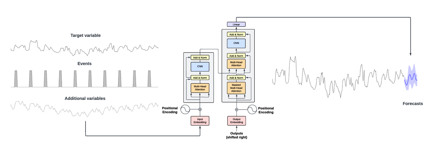
Source: 2310.03589 (arxiv.org) | TimeGPT takes the historical values of the target values and additional exogenous variables as inputs to produce the forecasts.
The TimeGPT model outperforms established statistical, machine learning, and deep learning methods, showcasing superior zero-shot inference performance, efficiency, and simplicity. As demonstrated in the benchmark below, TimeGPT excels across various machine learning metrics even without any feature engineering.
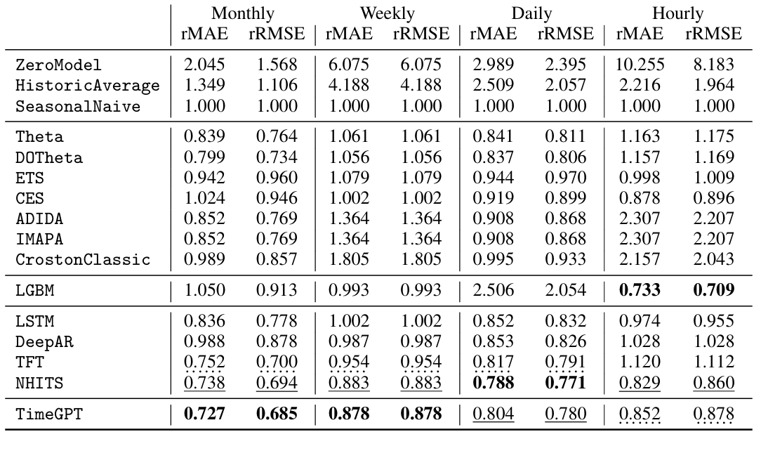
Source: 2310.03589 (arxiv.org) | Benchmark models measured with rMAE and rRMSE, lower scores are better.
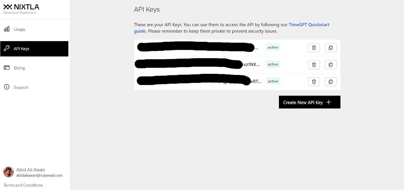
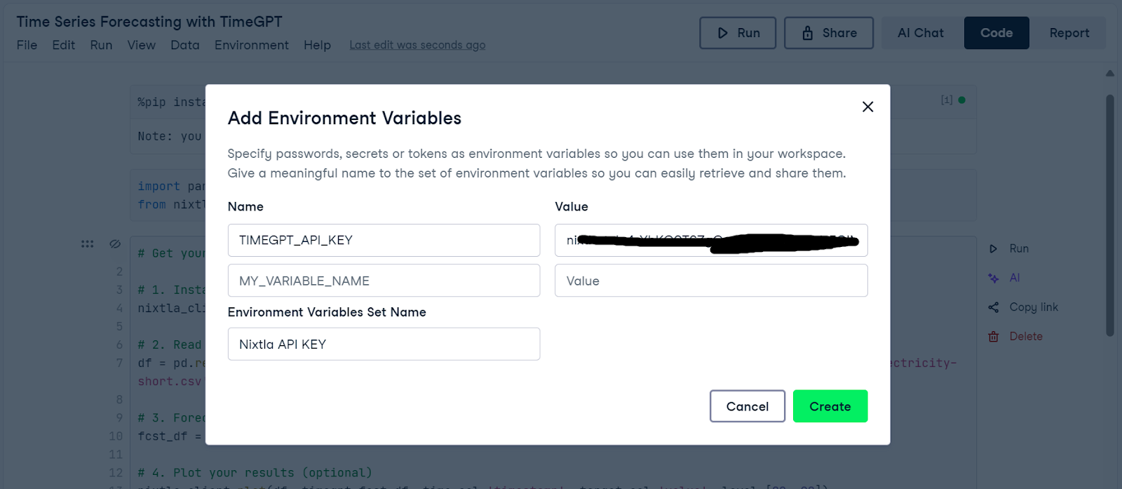
The TimeGPT model is not open source, and you can only access it through the Nixtla API. This section will guide you through setting up the Nixtla API to access the TimeGPT model and forecast Amazon stock data.
%%capture
%pip install nixtla>=0.5.1
%pip install yfinanceimport pandas as pd
import yfinance as yf
from nixtla import NixtlaClient
import os
timegpt_api_key = os.environ["TIMEGPT_API_KEY"]
# Setup NixtlaClient
nixtla_client = NixtlaClient(api_key = timegpt_api_key)
# Downloading Amazon stock price data
ticker = 'AMZN'
amazon_stock_data = yf.download(ticker)
amazon_stock_data = amazon_stock_data.reset_index()
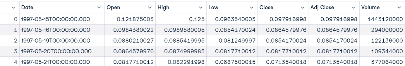
# Displaying the dataset
amazon_stock_data.head()We have Amazon stock price data starting from 1997 to the present.
nixtla_client.plot(amazon_stock_data, time_col='Date', target_col='Close')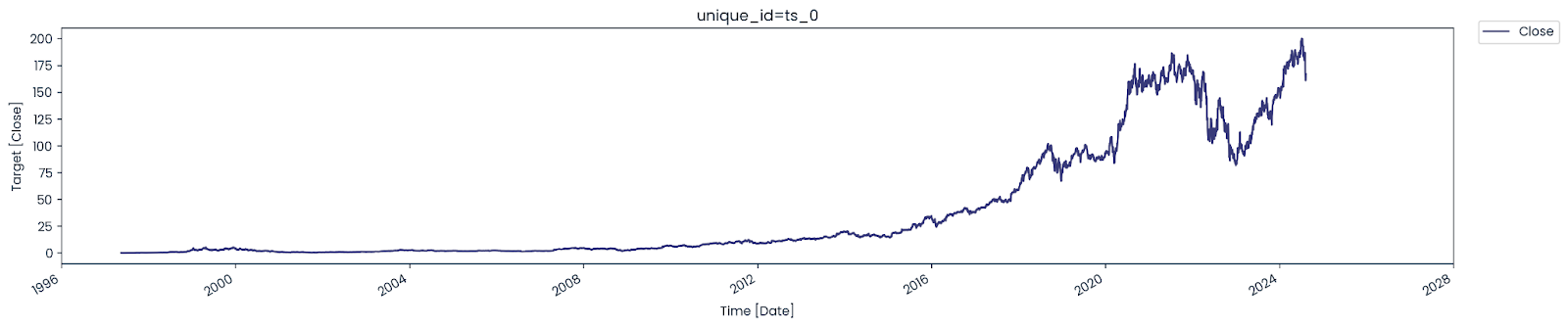
Discover how to create time series line plots using Matplotlib by following this Matplotlib Time Series Line Plot tutorial.
.forecast function with the stock data, model name, a forecast horizon (equivalent to 24 days), frequency, time columns, and target columns. Since the stock exchange is closed on weekends, we select the frequency as "business day(B)".model = nixtla_client.forecast(
df=amazon_stock_data,
model="timegpt-1",
h=24,
freq="B",
time_col="Date",
target_col="Close",
)
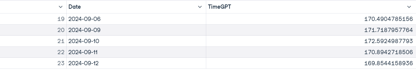
model.tail()
nixtla_client.plot(
    amazon_stock_data,
    model,
    time_col="Date",
    target_col="Close",
    max_insample_length=60,
)
As we can see, within a few seconds, the TimeGPT model accurately predicted Amazon's close prices into the future.
This was a beginner's example. In the next session, we will work on more complex datasets and explore various features of the Nixtla API.
In this section, we will use a more complex dataset of Australian Electricity Demand and use the TimeGPT model to forecast multiple values at once.
The dataset comprises 5 time series that represent the half-hourly electricity demand of 5 states in Australia: Victoria, New South Wales, Queensland, Tasmania, and South Australia.
We will also learn how to fine-tune the model and use various model hyperparameters to enhance performance. Finally, we will conduct cross-validation and compare the model's performance with traditional models to make a thorough assessment.
There is no simple way to load the .tsf file in the pandas library. We have to create our own custom function to load and process the data and then convert it into a Pandas dataframe.
import pandas as pd
def read_tsf_from_file(file_path):
data = []
start_date = pd.to_datetime("2002-01-01 00:00:00")
# Open and read the file from the directory
with open(file_path, "r") as file:
for line in file:
if line.startswith("T"):
parts = line.strip().split(":")
unique_id = parts[0] + "-" + parts[1]
values = list(map(float, parts[3].split(",")[:-1]))
# Generate datetime index at half-hour intervals
periods = len(values)
date_range = pd.date_range(
start=start_date, periods=periods, freq="30min"
)
# Append to data list
for dt, value in zip(date_range, values):
data.append([unique_id, dt, value])
# Convert the list of data into a DataFrame
return pd.DataFrame(data, columns=["unique_id", "ds", "y"])
# Example usage
file_path = "australian_electricity_demand_dataset.tsf"
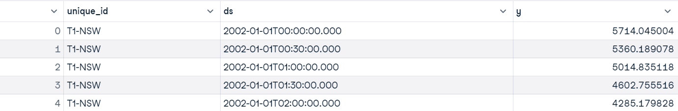
demand_df = read_tsf_from_file(file_path)
# Display the dataframe
demand_df.head()
Our dataset has three columns:
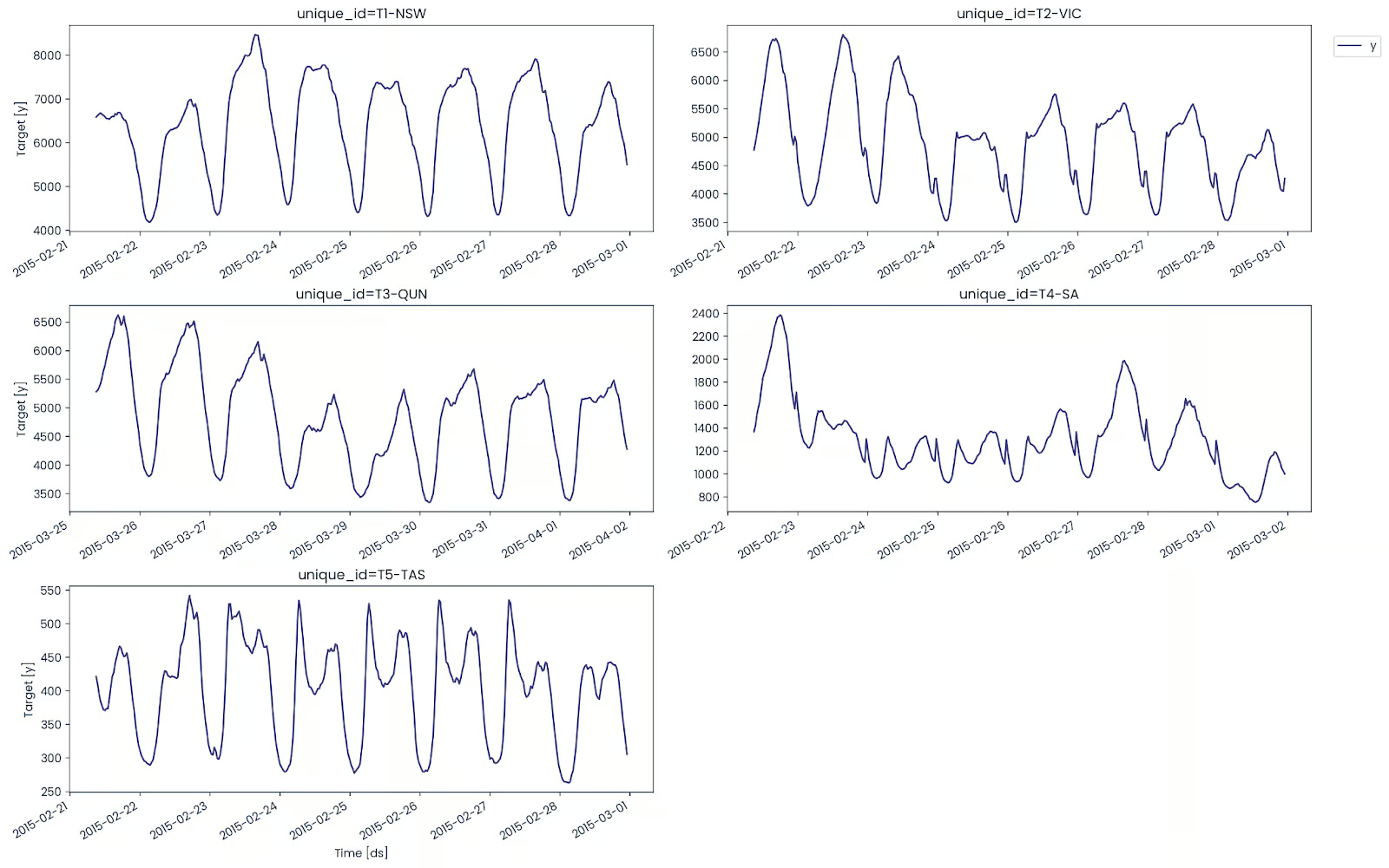
The plot function is excellent as it automatically identifies the unique_id column and creates five different time series visualizations.
nixtla_client.plot(
    demand_df,
    max_insample_length=365,
)
The visualization below shows the power consumption of 5 states, and they all have different patterns.
Learn time series analysis by participating in the live code-along session on DataCamp, where you will dive into financial time series datasets using Python.
In this session, we will explore various stocks, visualize their performance, and make forecasts using different models.
Before we forecast, we will identify various anomalies in the dataset to understand the problem better.
The .detect_anomalies function takes the dataset, time and target columns, and frequency.
# Detect anomalies
anomalies_df = nixtla_client.detect_anomalies(
    demand_df,
    time_col='ds',
    target_col='y',
    freq='H',
)
anomalies_df[anomalies_df["anomaly"]==1].head()
We have displayed all the instances where anomalies were detected.
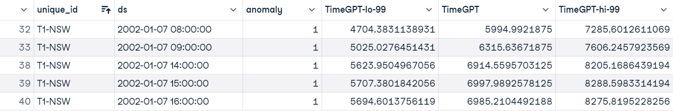
The total number of anomalies in all 5 time series datasets is 17,316, which is a a lot.
anomalies_df.anomaly.value_counts()
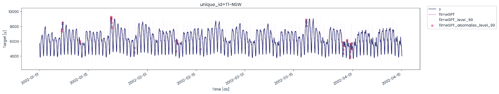
Now, we will plot the anomalies on the actual dataset to see where and how often they occur from day to day. To simplify the visualization, we will only display 5,000 samples from New South Wales.
# Plot anomalies
nixtla_client.plot(
    demand_df[demand_df["unique_id"]=="T1-NSW"][0:5000],
    anomalies_df[anomalies_df["unique_id"]=="T1-NSW"][0:5000],
    time_col='ds',
    target_col='y',

)
The anomalies on a daily basis are not common, but there have been days when multiple anomalies occur in a single day.
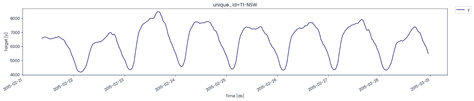
We will now forecast the New South Wales electricity demand. For that, we will filter out only the values for "T1-NSW".
T1_df = demand_df[demand_df["unique_id"]=="T1-NSW"]
T1_df.head()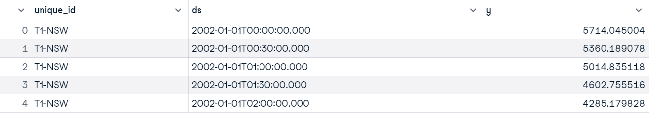
Plot the latest 365 values to understand the electrical consumption pattern.
nixtla_client.plot(
    T1_df,
    max_insample_length=365,
)
We will now evaluate our model's performance. To do so, we need to split our dataset into training and testing sets.
The training set consists of 144 values, which equates to 3 days, and the testing set consists of 1200 values, which equates to 25 days.
test_df = T1_df.tail(144) # 3 days = (144 * 0.5h *  1 day/24h)
train_df = T1_df.iloc[-1344:-144] # 25 days = (1200 *0.5h * 1 day/24h)
For forecasting, we will select a better model and set various arguments to improve model performance, specifically:
predict_df = nixtla_client.forecast(
    df=train_df,
    h=144,
    level=[90],  # Generate a 90% confidence interval
    finetune_steps=60,  # Specify the number of steps for fine-tuning
    finetune_loss="mae",  # Use the MAE as the loss function for fine-tuning
    model="timegpt-1-long-horizon",  # Use the model for long-horizon forecasting
    time_col="ds",
    target_col="y",
)
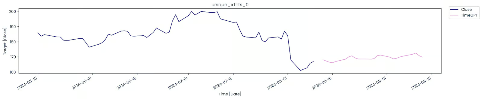
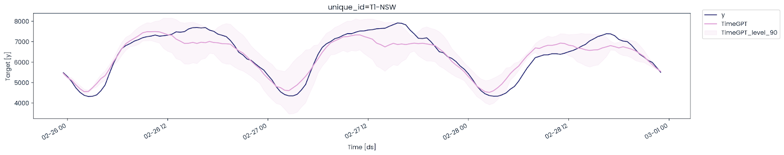
Plot the actual, forecast, and 90 percent confidence interval to assess the model's performance.
nixtla_client.plot(
    test_df, predict_df, models=["TimeGPT"], level=[90], time_col="ds", target_col="y"
)
Within a few seconds, we got a fairly accurate result. That is the power of pre-trained models.
We will now evaluate the model performance using the UtilsForecast library, which is part of the Nixtla open-source project. To do this, we will merge the test and forecast datasets and then provide them to the evaluate function. The function takes the dataset, metrics, models, target columns, and a unique ID to calculate the model metrics and display them as a pandas data frame.
from utilsforecast.losses import mae, rmse, smape
from utilsforecast.evaluation import evaluate
predict_df["ds"] = pd.to_datetime(predict_df["ds"])
test_df = pd.merge(test_df, predict_df, "left", ["ds", "unique_id"])
evaluation = evaluate(
test_df,
metrics=[mae, rmse, smape],
models=["TimeGPT"],
target_col="y",
id_col="unique_id",
)
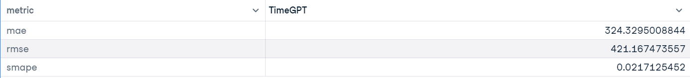
average_metrics = evaluation.groupby("metric")["TimeGPT"].mean()
average_metricsWe got fairly good results.
The Nixtla API also allows you to forecast multiple series at once. We will use the entire dataset instead of filtering based on a unique ID.
To split the dataset into the train and test sets, we use the groupby function to split the 144 values for each unique ID. Otherwise, we would have only 144 values for some randomly chosen unique ID.
values for some randomly chosen unique ID.
test_df = demand_df.groupby("unique_id").tail(144)  # 3 days
train_df = (
    demand_df.groupby("unique_id")
    .apply(lambda group: group.iloc[-1344:-144])
    .reset_index(drop=True)
)  # 25 days
The forecast function is the same as in the previous part, except this time, we are also including the ID columns.
predict_df = nixtla_client.forecast(
df=train_df,
h=144,
level=[90],
finetune_steps=60,
finetune_loss='mae',
model='timegpt-1-long-horizon',
time_col='ds',
target_col='y',
id_col='unique_id'
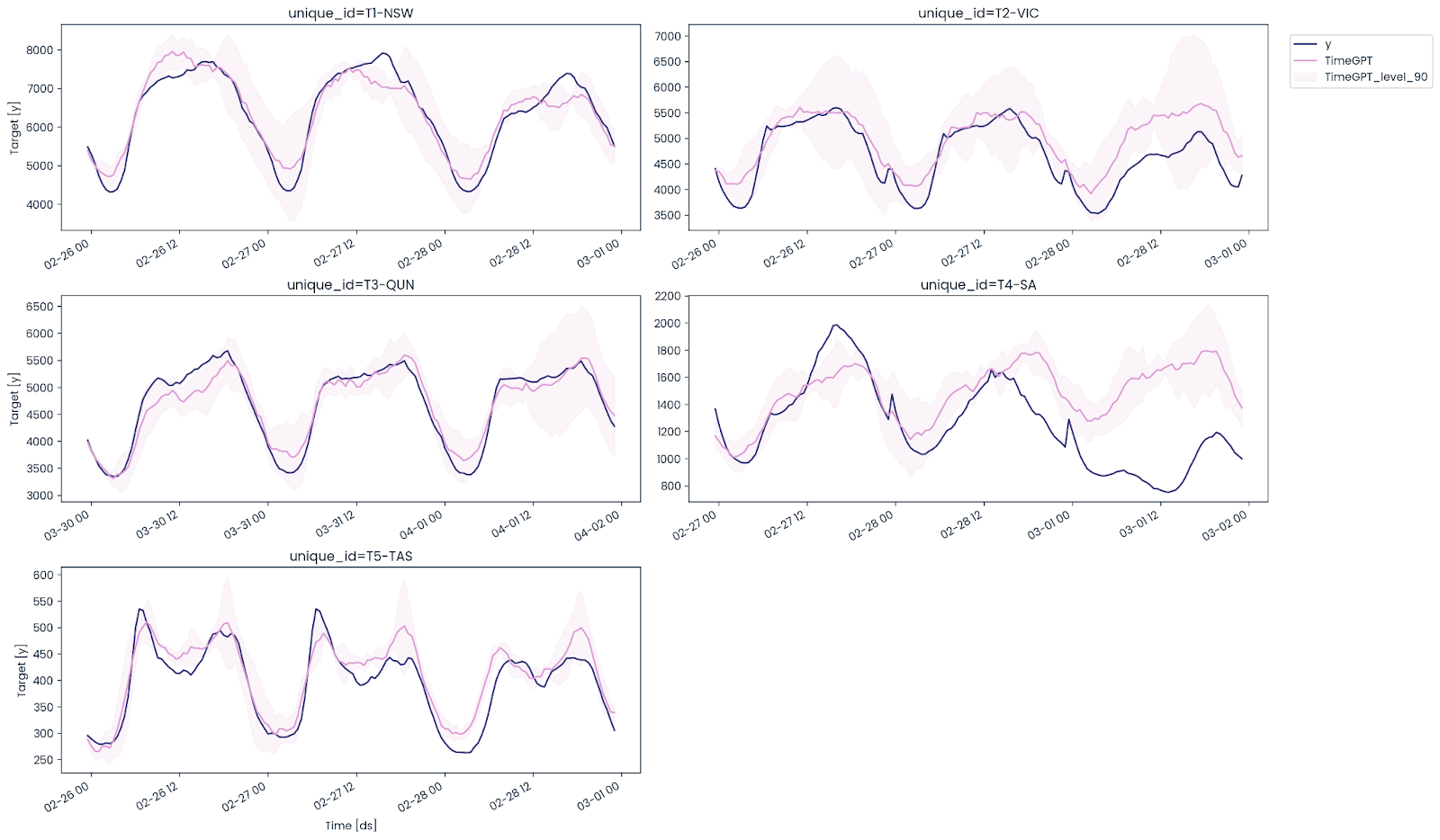
)Plot time series graph of actual, forecast, and 90 confidence level values of all 5 Unique IDs.
nixtla_client.plot(
    test_df, predict_df, models=["TimeGPT"], level=[90], time_col="ds", target_col="y"
)
As we can see, the TimeGPT model has performed well even on multiple time series, except for South Australia. It couldn't forecast the downward trend in electricity demand.
We need to merge the test and forecast dataframes to evaluate the model using MAE, RMSE, and SMAPE metrics.
predict_df['ds'] = pd.to_datetime(predict_df['ds'])
test_df = pd.merge(test_df, predict_df, 'left', ['ds','unique_id'])
Use evaluate function to generate a model performance report as a pandas dataframe. It will contain model metrics for each unique ID. To calculate the overall performance of the model, we have to average the values and display the final result.
evaluation = evaluate(
test_df,
metrics=[mae, rmse, smape],
models=["TimeGPT"],
target_col="y",
id_col = "unique_id"
)
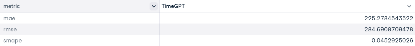
average_metrics = evaluation.groupby('metric')["TimeGPT"].mean()
average_metricsOverall model performance improves when fine-tuned on multiple time series instead of a single one.
The Nixtla client also allows you to perform cross-validation to evaluate model performance on various windows of the dataset.
We will use the .cross_validation function and provide it with the filtered dataset that contains only New South Wales values. The cross-validation will have 5 windows, each with a length of 7 hours.
timegpt_cv_df = nixtla_client.cross_validation(
T1_df,
h=7,
n_windows=5,
time_col='ds',
target_col='y',
freq='H',
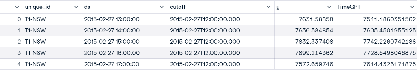
)
timegpt_cv_df.head()As we can see, we got forecast values based on the five 7-hour windows.
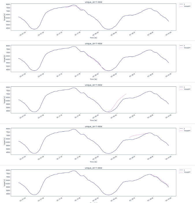
We will use a cutoff date and time to create 5 windows, each showing predicted and actual values.
cutoffs = timegpt_cv_df['cutoff'].unique()
for cutoff in cutoffs:
    fig = nixtla_client.plot(
        T1_df.tail(100),
        timegpt_cv_df.query('cutoff == @cutoff').drop(columns=['cutoff', 'y']),
        time_col='ds',
        target_col='y'
    )
    display(fig)
Apart from the 3rd and 4th splits, the model has performed quite well.
Let's now compare the performance of the TimeGPT and Light Gradient-Boosting Machine (LGBM) models to clearly determine which one excels on the same dataset. We have already performed cross-validation on the New South Wales dataframe; the next step is to use the evaluate function to generate the model evaluation report.
evaluation = evaluate(
    timegpt_cv_df,
    metrics=[mae, rmse, smape],
    models=["TimeGPT"],
    target_col="y",
    id_col = "cutoff"
)
evaluation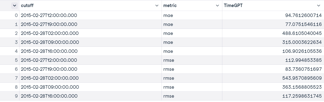
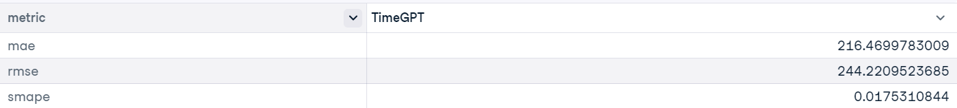
We need to calculate the mean of MAE, RMSE, and SMAPE for all 5 windows in order to obtain the overall result of the model.
average_metrics = evaluation.groupby('metric')["TimeGPT"].mean()
average_metrics
The results are quite good, even on a small set of values.
To evaluate the LGBM model, we need to follow these steps:
Note: To use statistical and machine learning models for time series forecasting, it's essential to learn the basic feature engineering techniques and algorithms. For a comprehensive guide on these topics, check out this tutorial: Time Series Forecasting Tutorial on DataCamp.
import pandas as pd
import numpy as np
import lightgbm as lgb
from sklearn.model_selection import TimeSeriesSplit
from sklearn.metrics import mean_absolute_error, mean_squared_error
# Function to calculate SMAPE
def smape(y_true, y_pred):
return np.mean(2 * np.abs(y_pred - y_true) / (np.abs(y_true) + np.abs(y_pred)))
# Assuming 'ds' is the date/time column and 'y' is the target variable
T1_df['ds'] = pd.to_datetime(T1_df['ds'])
# Filter the DataFrame to include only the specified datetime range
start_date = '2015-02-27T13:00:00'
end_date = '2015-02-28T23:00:00'
T1_df = T1_df[(T1_df['ds'] >= start_date) & (T1_df['ds'] <= end_date)]
# Convert 'ds' to a numerical value (e.g., timestamp)
T1_df['ds_num'] = T1_df['ds'].apply(lambda x: x.timestamp())
# Create lag and window features
for lag in range(1, 4):
T1_df[f'lag_{lag}'] = T1_df['y'].shift(lag)
T1_df['rolling_mean'] = T1_df['y'].rolling(window=3).mean()
T1_df['rolling_std'] = T1_df['y'].rolling(window=3).std()
# Drop NaN values resulting from lag and rolling operations
T1_df.dropna(inplace=True)
# Select features for the model
X = T1_df[['ds_num', 'lag_1', 'lag_2', 'lag_3', 'rolling_mean', 'rolling_std']]
y = T1_df['y']
# Time series split
tscv = TimeSeriesSplit(n_splits=5)
mae_scores = []
rmse_scores = []
smape_scores = []
for train_index, test_index in tscv.split(X):
X_train, X_test = X.iloc[train_index], X.iloc[test_index]
y_train, y_test = y.iloc[train_index], y.iloc[test_index]
# Initialize and train the LGBM model
model = lgb.LGBMRegressor(force_row_wise=True, verbosity=-1)
model.fit(X_train, y_train)
# Make predictions
y_pred = model.predict(X_test)
# Evaluate the model
mae = mean_absolute_error(y_test, y_pred)
rmse = np.sqrt(mean_squared_error(y_test, y_pred))
smape_value = smape(y_test, y_pred)
mae_scores.append(mae)
rmse_scores.append(rmse)
smape_scores.append(smape_value)
# Convert the metrics into a DataFrame
mae_avg = np.mean(mae_scores)
rmse_avg = np.mean(rmse_scores)
smape_avg = np.mean(smape_scores)
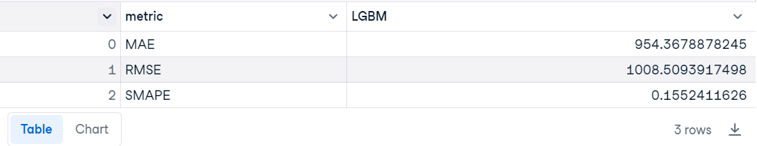
metrics_df = pd.DataFrame({
'metric': ['MAE', 'RMSE', 'SMAPE'],
'LGBM': [mae_avg, rmse_avg, smape_avg]
})
# Display the DataFrame
metrics_dfTimeGPT is almost 5 times better than LGBM.
If you are facing issues running the above code or setting up TimeGPT, please check out the DataLab workspace: Time Series Forecasting with TimeGPT.
The TimeGPT and Nixtla ecosystem is ideal for companies just starting out, as it eliminates the need to hire machine learning engineers to train models and MLOps engineers to deploy and maintain them. If you're a startup, you can save significantly on costs while still accessing high-performing models.
Similar to GPT-3, TimeGPT represents the beginning of state-of-the-art models for time series, and as these models improve over time, many companies are likely to adopt the Nixtla API for easy integration and enhanced performance.
In this tutorial, we have explored TimeGPT, the first foundational model for time series. Additionally, we have learned how to use the Python API to access the TimeGPT model for tasks such as forecasting, time series visualization, model evaluation, cross-validation, and anomaly detection.
Learn how to forecast the future using ARIMA class models and generate predictions and insights using machine learning models with the Time Series with Python skill track. If you prefer R language, consider the Time Series with R skill track to comprehensively understand time series forecasting.
Top DataCamp Courses
Track
Track
Track
blog
Sandra Kublik
15 min
Tutorial
Moez Ali
Tutorial
Moez Ali
Tutorial
Zoumana Keita
code-along
Richie Cotton
code-along
Zoumana Keita