Curso
Principios de ingeniería de software en Python
4 h
66.8K
Have you ever been asked how long a software project will take and realized your best answer was basically a guess?
That is how most teams approached software engineering cost estimation in the 1970s. Projects ran over budget and past deadlines regularly, and the methods in use, mostly expert judgment and rough analogies, did not hold up as systems grew larger and more complex.
COCOMO was built to fix that. It stands for COnstructive COst MOdel. Barry W. Boehm introduced it in his 1981 book Software Engineering Economics, basing the formulas on real project data rather than intuition. It became one of the most widely taught algorithmic estimation models in the field. Boehm, who passed away in August 2022, spent decades refining the ideas behind it.
In this tutorial, I'll walk you through how the model works, what the different types and levels mean, and run a full numerical example so the numbers make sense in practice.
COCOMO is a parametric software cost estimation model. It takes one primary input, specifically the estimated size of a software project measured in Thousands of Lines of Code (KLOC), and uses that to predict three things: total effort in person-months (PM), development time in months, and the number of people needed.
The model assumes that project size is the primary predictor of effort. Boehm built the model's constants by running regression analysis on real historical project data.
That said, COCOMO does not estimate monetary cost directly. It estimates effort. To convert person-months into dollars, you multiply by the average labor cost per person-month at your organization. The model gives you the effort; you supply the rate.
Boehm was working as Director of Software Research and Technology at TRW Aerospace, and the frustration was immediate and practical. According to a tribute later published by the National Academy of Engineering, a TRW vice president told Boehm after reviewing a competitive software bid: "I never want to have to sign off on another software bid based just on faith. Go and invent a way credibly to estimate the cost of developing a software product."
That request became COCOMO. Boehm studied 63 completed projects at TRW, spanning software ranging from 2,000 to 100,000 lines of code, written in languages from assembly to PL/I, all built under the waterfall model. The regression analysis on that dataset produced the constants used in COCOMO I, and the model went public in 1981.
The math behind Basic COCOMO I is simple once you understand what each term represents.
The effort formula is:
![]()
Here, effort is measured in person-months, KLOC is the estimated software size in thousands of lines of code, and a and b are constants that depend on the type of project you are working on.
The development time formula follows from the effort estimate:
![]()
The constant d varies by mode, while c is fixed at 2.5 across all three. Many tutorials get this wrong by implying all four constants change. Once you have both Effort and , you can estimate the average number of people required:

The table below shows the verified constants for Basic COCOMO I:
|
Project Mode |
a |
b |
c |
d |
|
Organic |
2.4 |
1.05 |
2.5 |
0.38 |
|
Semi-Detached |
3.0 |
1.12 |
2.5 |
0.35 |
|
Embedded |
3.6 |
1.20 |
2.5 |
0.32 |
The key variable here is b. For Organic projects, b = 1.05, which means effort grows nearly linearly with project size. For Embedded projects, b = 1.20, which creates a significant diseconomy of scale: doubling the size of an embedded project more than doubles the required effort.
COCOMO I categorizes software projects into three development modes. Each mode reflects a different combination of team experience, project complexity, and operational constraints. The mode you choose determines which constants go into your formulas.
Worth noting upfront: these three modes apply only to COCOMO I. COCOMO II, the 2000 update, replaced them with a different approach.
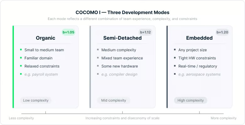
Three COCOMO I modes compared visually. Image by Author.
The three modes sit on a scale of increasing complexity and constraint. Your project type and team context will usually make it clear which one applies.
Organic mode covers small to medium projects where the team has solid experience with the application domain, requirements are relatively well understood, and there is no significant external pressure from hardware constraints or regulatory requirements. A payroll system, a data processing application, or an inventory management tool would typically fall here.
Because the team is experienced and the domain is familiar, communication overhead stays low even as the project grows. That is why the b exponent is the smallest of the three modes.
Semi-detached mode sits in the middle. Teams in this category have mixed experience: some members know the domain well, others do not. The project has moderate complexity, and there may be some interaction with new hardware or external systems.
Compiler development, transaction processing systems, and mid-tier business applications are common examples. The diseconomy of scale is more noticeable here, with b = 1.12.
Embedded mode applies to projects with tight operational constraints: strict hardware requirements, real-time processing demands, regulatory standards, or aerospace and defense requirements. The team may be large and technically skilled, but the complexity of integration, testing, and validation drives effort up sharply as project size increases.
With b = 1.20, embedded projects have the steepest diseconomy of scale of the three modes. Embedded mode is also not about project size. Even a relatively small embedded system qualifies if it operates under severe constraints.
Beyond the three project modes, COCOMO I has three levels of estimation detail. The modes tell you which constants to use; the levels tell you how deeply to model the project. Each level builds on the previous one by adding more factors to the calculation, which increases accuracy at the cost of more input data.
Think of it as a spectrum: Basic COCOMO gives you a fast ballpark figure, while Detailed COCOMO lets you do precise phase-level planning.
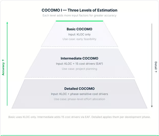
COCOMO I levels by estimation detail depth. Image by Author.
Moving down the pyramid adds more factors to the calculation, which increases accuracy but also requires more input data to get started.
Basic COCOMO uses only the project size in KLOC and the project mode. You plug in KLOC, apply the constants for your chosen mode, and get an effort estimate. This is useful for early feasibility assessments when you do not yet have detailed information about your team or development environment.
Intermediate COCOMO introduces an Effort Adjustment Factor, usually written as EAF. The full list of cost driver multipliers is documented in the COCOMO II Model Definition Manual. The effort formula becomes:
![]()
The EAF is the product of 15 cost drivers, each rated on a scale from Very Low to Extra High. The drivers fall into four categories: product attributes (reliability, complexity, database size), hardware attributes (execution time and storage constraints), personnel attributes (team experience and capability), and project attributes (tooling, schedule pressure, and development practices).
One thing to know about Intermediate COCOMO: the a constant changes from its Basic values. For Organic mode, a becomes 3.2 (not 2.4). For semi-detached mode, it stays at 3.0. For Embedded mode, it drops to 2.8. The b, c, and d exponents remain the same across both Basic and Intermediate levels.
Personnel cost drivers are inverted: higher capability means a smaller multiplier, which reduces the effort estimate. A team of experienced programmers simply does not need as many person-months to finish a project as a team of beginners.
Detailed COCOMO, sometimes called Advanced COCOMO, applies effort multipliers at the individual phase level rather than across the whole project. This means the cost drivers for requirements analysis, detailed design, coding, and integration and testing are evaluated separately.
This is the most accurate level, and also the most time-consuming to use. It makes sense for large projects where different teams own different phases and where the effort distribution across phases matters for planning.
By the mid-1990s, COCOMO I was showing its age. Software development had shifted from waterfall projects on mainframes to object-oriented programming, reusable component libraries, rapid prototyping, and distributed desktop systems. Applying 1970s project data to 1990s software environments was producing unreliable estimates.
Boehm and his colleagues at the USC Center for Software Engineering spent several years rebuilding the model from scratch. The result was COCOMO II, published in 2000 in the book Software Cost Estimation with COCOMO II, calibrated against a dataset of 161 projects, more than double the 63 from the original model.
The motivations behind COCOMO II were object-oriented and component-based development, software reuse and commercial off-the-shelf integration, iterative and spiral development models, and modern tooling. One common misconception worth clearing up: COCOMO II was not built for Agile development. Agile as we know it today barely existed when the model was being developed from 1995 to 2000.
COCOMO II offers three sub-models, each suited to a different phase of a project's life.
The Application Composition Model is designed for early prototyping, particularly when teams are using GUI builders and component libraries. Instead of KLOC, it uses Object Points: screens, reports, and third-generation language components weighted by complexity and adjusted for expected reuse. This is a linear model with no scale factors or exponential adjustments.
The Early Design Model is used before the architecture has been established. It takes Unadjusted Function Points as input, converts them to equivalent source lines of code using language-specific tables, and applies seven cost drivers. It gives a reasonable estimate when you know what the system should do but not yet how it will be built.
The Post-Architecture Model is the most rigorous of the three. It is deployed after the software architecture is settled, using Thousands of Source Lines of Code (KSLOC) or function points as input, 17 cost drivers, and five scale factors. The effort formula is:
![]()
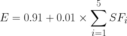
Where E is a dynamic exponent calculated as:
And the schedule formula is:
![]()
Where:
![]()
The constants 2.94, 0.91, 3.67, and 0.28 come from the COCOMO II.2000 calibration. Some older sources cite 2.5 instead of 2.94; that is a pre-2000 calibration value and should not be used with the current model. The USC COCOMO II Web Tool at softwarecost.org is a free, live implementation of the Post-Architecture model if you want to run estimates without doing the math manually.
Two mechanisms make COCOMO II work differently from COCOMO I: scale factors and cost drivers. Here is what each one does.
In COCOMO I, the exponent b is fixed by mode: you pick Organic, semi-detached, or Embedded, and you get a preset number. COCOMO II replaces this with five continuously-rated scale factors that calculate the exponent based on how you rate each one.
The five scale factors in COCOMO II are precedentedness (PREC), development flexibility (FLEX), architecture and risk resolution (RESL), team cohesion (TEAM), and process maturity (PMAT). Each is rated on a scale from Very Low to Extra High, and their combined sum determines E in the effort formula. A higher sum means a less mature, less familiar, riskier project, which means a higher exponent and more effort.
Scale factors affect the shape of the effort curve. Cost drivers, by contrast, are multiplicative adjustments applied to the baseline effort. COCOMO II has 17 cost drivers in the Post-Architecture model, compared to 15 in Intermediate COCOMO I. The additions in COCOMO II include factors for required reusability (RUSE), documentation requirements (DOCU), platform volatility (PVOL), personnel continuity (PCON), application experience (APEX), platform experience (PLEX), language and tool experience (LTEX), and multisite development (SITE).
One cost driver worth highlighting is SCED, which covers the required development schedule. If you compress a schedule significantly, the effort multiplier rises above 1.0, meaning you actually need more person-months to finish faster. This matches something most engineers already know from experience: forcing a team to sprint leads to coordination overhead, errors, and rework that often costs more than the time saved.
The model's primary strength is transparency. Unlike proprietary estimation tools, COCOMO publishes all its equations, constants, and calibration methodology. Anyone can audit the inputs and verify the outputs. This makes it useful in government, defense, and aerospace procurement, where mathematical auditability is often a legal or contractual requirement.
The model can also be recalibrated. Organizations that collect their own project history data can adjust the constants to reflect their specific environment, team composition, and technology stack. This is important because the default constants come from datasets that are now decades old.
The three-level structure (Basic → Intermediate → Detailed) is another practical benefit. Early in a project, when little is known, you use Basic for a rough estimate. As the project matures and more is understood about the team and environment, you move to Intermediate or Detailed for more refined planning.
The biggest limitation is COCOMO's dependency on KLOC. To use COCOMO, you need to estimate the size of a project in lines of code before you write any code. In the early stages of a project, exactly when estimation matters most, this is notoriously difficult to do accurately.
Even when KLOC can be estimated, the constants in COCOMO I come from 63 projects built under the waterfall model between 1968 and 1979. The constants in COCOMO II come from 161 projects from the 1990s. Neither dataset includes cloud-native systems, mobile applications, microservices architectures, or modern DevOps pipelines. Applying these constants directly to a modern project without local calibration produces unreliable estimates.
A 2025 study put numbers to this. An uncalibrated Basic COCOMO applied to a NASA project dataset produced an average relative error of approximately 100%, with no predictions falling within 25% of actual effort. That is not a small margin of error; it reflects a model being used outside the conditions it was built for.
The model also doesn't handle iterative development well. COCOMO assumes a reasonably sequential lifecycle. Agile teams working in short sprints with evolving backlogs do not fit the waterfall assumptions baked into COCOMO's structure.
There is also a deeper problem. A paper published in Frontiers in Artificial Intelligence in March 2026 argued that COCOMO II is fundamentally misaligned with AI-assisted software development, not just as a matter of calibration but structurally. When AI coding tools generate substantial portions of a codebase, KLOC as a proxy for human effort becomes misleading. The effort now centers on verification, architectural governance, and security review, none of which COCOMO's cost driver framework was designed to capture.
COCOMO is not the only option. Knowing the alternatives helps you pick the right approach for a given situation.
Function Point Analysis (FPA) measures system complexity from user-facing inputs and outputs, independent of programming language. It works well when you have solid requirements but no KLOC estimate yet. COCOMO II's Early Design model accepts function points as input, so the two can be used together.
Story Points are standard in Agile environments. Teams rate user stories by relative complexity, then track velocity to project progress. They are fast and team-specific, but do not produce the total-cost baseline that procurement and long-range planning require. COCOMO and story points serve different purposes.
Parametric tools like SEER-SEM and SLIM use proprietary calibration databases and broader parameter sets. Studies find they outperform uncalibrated COCOMO II on accuracy. COCOMO's advantage is transparency and open availability, which matters in academic or auditable contexts.
Machine learning-based estimation is an active research area. A January 2026 study found that ensemble models combining random forests, support vector regression, and neural network outperformed COCOMO-family models on Agile project data across all four standard evaluation metrics. These approaches adapt to their training data rather than relying on constants set decades ago.
Knowing where COCOMO fits relative to other methods is useful, but the best way to understand how it actually works is to run the numbers. Let's walk through a complete Basic COCOMO I calculation using Organic mode and a project estimated at 50 KLOC.
The constants for Organic mode are: a = 2.4, b = 1.05, c = 2.5, d = 0.38.
![]()
To compute 501.05, use the fact that 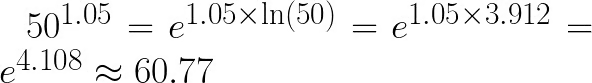 .
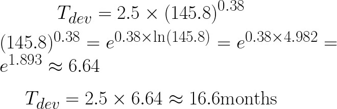
.
![]()

Summary:
|
Output |
Value |
|
Effort |
~145.8 person-months |
|
Development time |
~16.6 months |
|
People required |
~9 persons |
Two things worth noting. Person-months and calendar months are different units: 145.8 person-months over 16.6 calendar months means roughly 9 people working in parallel. And since this is Basic COCOMO, it uses only size and mode. Adding real cost driver ratings via EAF would shift the effort estimate up or down from there.
COCOMO comes up in academic courses, university exams, and interviews for roles in government, defense, and systems engineering. It rarely appears at agile consumer tech companies.
The most common question is COCOMO I versus COCOMO II: fixed modes and preset constants from 63 projects versus five continuous scale factors on a larger modern dataset. Knowing that distinction, the basic formulas, and the three mode names covers most scenarios. Interviewers occasionally ask for a sample calculation, so the worked example above is worth practicing.
COCOMO stays useful where its assumptions hold: sequential development, formal procurement, and academic study. Where modern software diverges from those conditions, it breaks down.
Use Basic COCOMO for a fast order-of-magnitude check early in a project. Use Intermediate COCOMO when you have team and environment data to work with. Calibrate to your own project history before relying on any output in a real bid or plan. As I covered in the Limitations section, applying the default constants to a modern project without calibration produces errors too large to act on.
COCOMO III has been in development at the Boehm CSSE since around 2015, with no public release as of March 2026. The 1981 original and its 2000 update remain the benchmark.
Want to go further with software development? We have courses on Software Engineering Principles in Python, Software Development with Cursor, and Software Development with GitHub Copilot to help you build what you’ve learned here.
Learn with DataCamp
Curso
Curso
Curso
blog
Kurtis Pykes
9 min
blog
Josep Ferrer
10 min
Tutorial
Khalid Abdelaty
Tutorial
Mark Pedigo
Tutorial
Bunmi Akinremi
Tutorial
Vikash Singh