Contrastive Learning: How Models Learn by Comparison

Getting a model to learn without labeled data sounds impossible, but that's the idea behind contrastive learning.

As you know, labeling data is slow and expensive. A single image classification dataset usually requires thousands of hours of human annotation, and that's before you account for errors and inconsistencies.

Contrastive learning goes around this labeling problem by teaching models to compare. So, instead of telling a model what something is, you show it what things are similar and what things are different - and let it figure out the rest.

In this article, I'll walk you through the intuition behind contrastive learning, how it works under the hood, where it's used in practice - from image recognition to NLP embeddings - and how to implement it in PyTorch.

What exactly is computer vision? Read our beginner guide to image analysis.

What Is Contrastive Learning?

Contrastive learning is an approach to training where a model learns by comparison instead of classification.

Instead of telling the model "this is a cat" or "this is a dog," you show it pairs of examples and let it figure out what belongs together and what doesn't. The model learns by figuring out if these two things are similar or not.

In other words - you feed the model two data points at a time. If they're related - say, two photos of the same dog taken from different angles - that's a positive pair. If they're unrelated - a photo of a dog and a photo of a car - that's a negative pair.

The model's job is to produce representations (numerical vectors) that follow this structure. Positive pairs should end up close together in vector space. Negative pairs should end up far apart.

Intuition Behind Contrastive Learning

The easiest way to understand contrastive learning is through images.

Take a photo of a dog. Now create two versions of it - one cropped, one with adjusted brightness. The content you see is the same, but the pixels are different. A contrastive learning model sees these two versions as a positive pair and learns to map them to similar positions in vector space.

If you show the model a photo of a car alongside that dog photo, you’ll get a negative pair. The model learns to push their representations apart.

You don’t need to manually intervene and specify "this is a dog" or "this is a car." The model builds its understanding from the structure of similarity and difference.

This is what makes contrastive learning powerful.

The signal comes from comparison. With enough pairs, the model can develop representations that understand what makes things alike and what sets them apart.

Those representations turn out to be genuinely useful. A model trained this way on images can be fine-tuned for classification, detection, or retrieval tasks with very little labeled data, because it's already learned something meaningful about the visual world.

Applications of Contrastive Learning

Contrastive learning shows up in many domains - here's where you'll see it the most.

Computer vision

This is where contrastive learning first proved what it can do.

Models trained this way on images learn to produce representations that understand visual similarity without ever seeing a label. Two photos of the same scene, shot from different angles or under different lighting, should map to nearby points in vector space. Two unrelated scenes should map far apart.

You can take a contrastively pre-trained model and fine-tune it for classification or object detection with a fraction of the labeled data you'd otherwise need.

Natural language processing

In NLP, contrastive learning is used to train sentence embeddings - vector representations that understand the meaning of a sentence as a whole.

Sentences with similar meanings should be close together in vector space, and unrelated sentences should be placed apart. Models trained this way can perform tasks like semantic search and sentence similarity, without large amounts of labeled sentence pairs.

Recommendation systems

Recommendation systems use contrastive learning to model user-item similarity.

A user and an item they've interacted with form a positive pair. A user and a random item they've never seen form a negative pair. If you train on enough of these, the model learns a shared space where relevant users and items cluster together.

Multimodal models

This is where contrastive learning gets interesting.

Models like CLIP use it to align text and images in a shared vector space. A photo of a dog and the sentence "a dog playing in the park" should end up close together. A photo of a dog and the sentence "a red sports car" should not. This lets multimodal models match images to text descriptions and generate captions.

How Contrastive Learning Works

Contrastive learning always follows the same four steps, regardless if you’re working with images, text, or audio.

Step 1: Create pairs

Every training example starts as a pair. You sample two data points and label the relationship as similar (positive) or dissimilar (negative). In practice, positive pairs often come from augmenting the same input in two different ways, and negative pairs come from sampling unrelated examples.

Step 2: Encode into embeddings

Both data points pass through an encoder that converts them into vectors. These vectors, called embeddings, are numerical representations that live in a shared vector space. The goal is for that space to reflect semantic meaning, and not raw pixel or token values.

Step 3: Compute similarity

Once you have two embeddings, you measure how close they are. Cosine similarity is the most common choice here. It gives you a score between -1 and 1, where 1 means the vectors point in the same direction and -1 means they're completely opposite.

Step 4: Update the model

The model compares its similarity scores against what they should be. For positive pairs, the score should be high. For negative pairs, it should be low. A loss function measures how far off the model is, and backpropagation adjusts the encoder weights to do better next time.

If you repeat these steps across enough pairs, the encoder will learn to produce embeddings that cluster similar things together and push different things apart.

Positive and Negative Samples

The quality of your contrastive model depends on how you create your pairs.

Positive pairs are two data points that should be considered similar. In computer vision, that usually means two augmented versions of the same image. In NLP, it might be two paraphrases of the same sentence, or a sentence and its translation. The model learns that whatever varies between them doesn't matter. The only thing that matters is what's shared.

Negative pairs are two data points that should be considered different. Most implementations sample negatives randomly from the rest of the dataset. If you're training on images, any two images of different objects make a valid negative pair.

Here's where it gets tricky.

Not all negatives are equally useful. A random negative that's obviously different from the source - say, a photo of a dog paired with a photo of an airplane - doesn’t make the model work very hard. These are called easy negatives, and training on too many of them slows learning down.

On the other side, hard negatives are data points that look similar to the source but belong to a different class - two dog breeds, for example, or two sentences with similar wording but different meanings. The model has to develop finer-grained representations to tell them apart, which produces better embeddings overall.

The same logic applies to positives. If your augmentations are too subtle, the model doesn't learn much. If they're too aggressive, the pair isn’t meaningfully similar anymore.

Contrastive Loss Functions

The loss function turns pair comparisons into learning signals.

Each loss function works differently, but they all share the same goal of rewarding the model when similar things are close in vector space, and penalizing it when they're not.

Contrastive loss

Contrastive loss was introduced alongside the early contrastive learning work.

It operates on pairs. Given a positive pair, it penalizes the model if their embeddings are far apart. Given a negative pair, it penalizes the model if their embeddings are too close - specifically, if they fall within a defined margin. Negatives that are already far enough apart don't contribute to the loss.

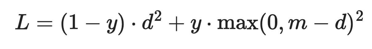
Contrastive loss formula

Where d is the distance between two embeddings, y is 1 for negative pairs and 0 for positive pairs, and m is the margin. The margin is a hyperparameter you set manually, which makes this loss sensitive to tuning.

Triplet loss

Triplet loss works with three data points at once: an anchor, a positive, and a negative.

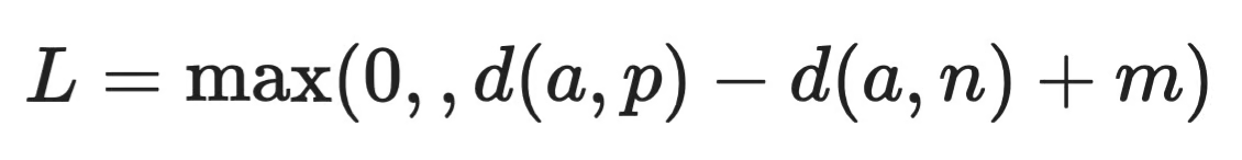
Triplet loss formula

The model is penalized whenever the anchor-to-positive distance d(a, p) isn't smaller than the anchor-to-negative distance d(a, n) by at least margin m. If that condition is already met, the loss is zero.

This formulation gives the model more context per update than contrastive loss, because it's comparing both relationships at once rather than one at a time.

InfoNCE loss

InfoNCE is the loss behind most modern contrastive learning methods, including SimCLR and CLIP.

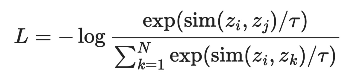
InfoNCE loss formula

For each anchor z_i, the model has to identify its positive z_j from all other N examples in the batch. The temperature parameter τ controls how sharp the distribution is - lower values make the model more confident, higher values soften the contrast between pairs.

You get more negatives per update, which gives the model more learning signal. It also means that larger batches expose the model to harder negatives and generally produce better representations.

Contrastive Learning in Self-Supervised Learning

Contrastive learning and self-supervised learning work well together, and by understanding why, you’ll understand where modern ML is heading.

Self-supervised learning is a training approach where the model generates its own labels from the data, without human annotation. So instead of someone labeling thousands of images as "cat" or "dog," the data itself provides the supervision signal.

Contrastive learning does exactly that. When you take an image, create two augmented versions of it, and tell the model they're a positive pair, you've just created a label.

This matters because labeled data is the bottleneck in most ML pipelines. Collecting it is slow, annotation is expensive, and some domains, such medical imaging, don't have enough of it.

The results so far have been promising. Models pre-trained with contrastive self-supervised objectives on large unlabeled datasets have matched or come close to supervised baselines on a range of downstream tasks, after fine-tuning on only a small amount of labeled data.

The general trend is to move away from task-specific supervised training and toward general-purpose representations learned from raw data at scale. Methods like SimCLR, MoCo, and BYOL all follow this trend, and I’ll discuss them next.

Popular Contrastive Learning Methods

Here are the three most influential frameworks behind contrastive learning in 2026.

SimCLR

SimCLR, introduced by Google Research, is one of the clearest implementations of the contrastive learning idea.

For each image in a batch, it creates two augmented views and treats them as a positive pair. Every other image in the batch becomes a negative. The model, which is a CNN followed by a small projection head, learns to map positive pairs close together using InfoNCE loss.

What made SimCLR stand out was how much batch size mattered. Larger batches meant more negatives per update, which translated to better representations. The tradeoff is memory. As SimCLR requires large batches to work well, you need good hardware to get the most out of it.

MoCo

MoCo (Momentum Contrast), from Meta AI Research, was designed to solve exactly that problem.

Instead of relying on a large batch for negatives, MoCo maintains a queue - a running buffer of encoded representations from previous batches. This decouples the number of negatives from batch size, so you can train with far less memory and still expose the model to a large pool of negatives.

It also uses a momentum encoder, which is a slowly updated copy of the main encoder, to keep the representations in the queue consistent over time.

BYOL

BYOL (Bootstrap Your Own Latent) is worth mentioning here even though it doesn't use negative pairs at all.

Instead of pushing negatives apart, BYOL trains one network to predict the representations of another - a slowly updated target network. There are no negatives and no contrastive loss. It works surprisingly well, and its success challenged the assumption that negative pairs are necessary for contrastive-style learning.

BYOL is somewhere on the edge of contrastive learning, but it's a good next step once you understand how the core methods work.

Contrastive Learning vs Supervised Learning

These two approaches solve the same problem, but they start from different assumptions that you need to understand.

Supervised learning requires labeled data. Every training example needs a human-assigned label, and the model learns by mapping inputs to those labels. It's a direct approach, and it works well when you have enough labeled examples. The model knows what the input is and what the correct answer is.

Contrastive learning generates its own supervision from the structure of the data - similarity and difference - and learns representations without ever seeing a label.

Here's a more visual representation of how they compare:

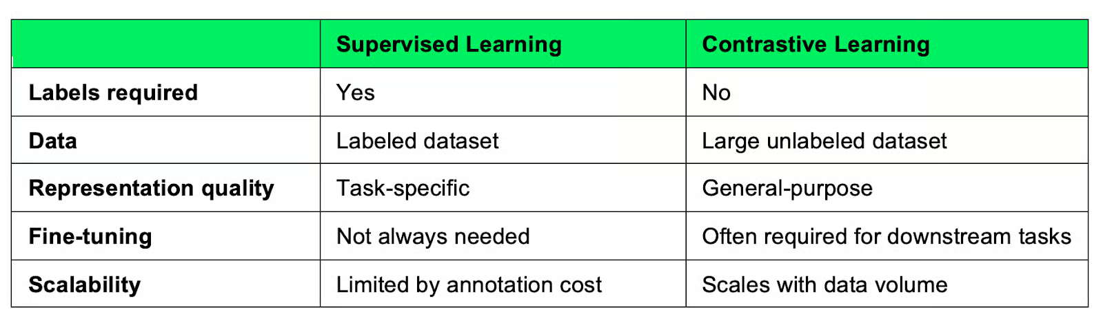
Contrastive learning compared to supervised learning

Most of the difference shows at scale. Supervised learning is dependent on labeled data - and labeling more is expensive. Contrastive learning can keep improving as you feed it more unlabeled data, which is usually abundant.

But it’s important to note the representations contrastive learning model learns are general, not task-specific, which means you'll usually need a fine-tuning step to get good performance on a specific task. Supervised models don’t need that step because they're trained on the target objective.

The choice comes down to your data situation. If you have labeled data and a specific task, supervised learning is often faster. If you're working with large amounts of unlabeled data or need representations that transfer across tasks, contrastive learning can be worth the extra setup.

Contrastive Learning in Practice (Python Example)

Let me now make a minimal PyTorch implementation. The example below covers the three core ideas discussed earlier: an embedding model, cosine similarity, and NT-Xent loss - the loss function used in SimCLR, built on top of InfoNCE.

The embedding model

The encoder is a simple feedforward network that maps input vectors to a lower-dimensional embedding space.

import torch
import torch.nn as nn
import torch.nn.functional as F

class Encoder(nn.Module):
    def __init__(self, input_dim, embedding_dim):
        super().__init__()
        self.network = nn.Sequential(
            nn.Linear(input_dim, 128),
            nn.ReLU(),
            nn.Linear(128, embedding_dim)
        )

    def forward(self, x):
        return self.network(x)

In practice, you'd replace this with a CNN for images or a transformer for text. The architecture matters less than what comes after it.

Similarity computation

Once you have two embeddings, you measure how close they are using cosine similarity. Normalizing the vectors first keeps the similarity scores bounded between -1 and 1.

def cosine_similarity(z1, z2):
    z1 = F.normalize(z1, dim=-1)
    z2 = F.normalize(z2, dim=-1)
    return torch.matmul(z1, z2.T)

The result is a matrix where each entry [i, j] represents the similarity between embedding i and embedding j across the batch.

NT-Xent loss

NT-Xent (Normalized Temperature-scaled Cross Entropy) is the InfoNCE-based loss. For each anchor, it treats its paired view as the positive and all other examples in the batch as negatives.

def nt_xent_loss(z1, z2, temperature=0.5):
    batch_size = z1.shape[0]

    z = torch.cat([z1, z2], dim=0)
    z = F.normalize(z, dim=-1)
    sim_matrix = torch.matmul(z, z.T) / temperature

    mask = torch.eye(2 * batch_size, dtype=torch.bool)
    sim_matrix = sim_matrix.masked_fill(mask, float("-inf"))

    labels = torch.arange(batch_size)
    labels = torch.cat([labels + batch_size, labels])

    return F.cross_entropy(sim_matrix, labels)

The temperature parameter controls how sharp the distribution is. Lower values make the model more confident about which pair is positive; higher values soften the contrast.

Putting it together

encoder = Encoder(input_dim=64, embedding_dim=32)
optimizer = torch.optim.Adam(encoder.parameters(), lr=1e-3)

# Simulate a batch of positive pairs
x1 = torch.randn(32, 64)
x2 = torch.randn(32, 64)

# Training
optimizer.zero_grad()
z1, z2 = encoder(x1), encoder(x2)
loss = nt_xent_loss(z1, z2)
loss.backward()
optimizer.step()

print(f"Loss: {loss.item():.4f}")

Contrastive loop output

This is the full contrastive loop in its simplest form. In a real implementation, x1 and x2 would be two augmented views of the same input instead of random noise - but the structure stays exactly the same.

Conclusion

Contrastive learning is a simple idea with a lot of reach.

It teaches models to understand structure through comparison instead of relying on labeled data. Push similar things together, pull different things apart - that's the whole premise, It turns out to be enough to learn representations that transfer well across tasks.

The field is moving away from annotation-heavy pipelines, and contrastive learning is a big reason why. Algorithms like SimCLR, MoCo, and CLIP made it into real products, which says something about how well the approach actually works.

If you want to go deeper, a good next step is getting your hands on a real implementation. The PyTorch example in this article is a starting point, but running SimCLR on an actual image dataset - even a small one - will teach you more than any explanation can.

And if you need the ultimate resource to advanced machine learning topics, enroll in our Machine Learning Scientist in Python track.